Random Numbers
Menu location: Data_Generating_Random Numbers.
This function enables you to create one or more series of random numbers from given distributions.
A robust generator of uniform (pseudo)random numbers is used as the basis for generating deviates from the probability distributions described below. You are given the opportunity to enter your own seed number to be used by the random number generator but you should use the default seed (based upon your computer's clock) in most cases. Please note that each seed generates its own series and that series is the same if you use the seed again. You have very little chance of using the same seed twice if you select the seed that StatsDirect suggests.
These functions are intended for simulation work; they employ widely cited and debated algorithms (Gentle, 2003).
Uniform (continuous uniform, rectangular)
The continuous uniform distribution has a constant density function of the interval (a, b) and thus a rectangular shape from a to b:
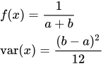
- where a and b lie between minus and plus infinity.
The interval most commonly used is 0 to 1
For an interval a to b, StatsDirect asks for the number type: interval (any value between a and b) or count (whole numbers from a to b inclusive, each equally likely).
Normal (Gaussian)
The commonly used standard normal distribution (mean of 0 and standard deviation of 1) is one of a family of normal distributions defined by the density function:

- where mean μ lies between minus and plus infinity and standard deviation σ is greater than zero.
Algorithm: inversion of the cumulative distribution function (Wichura, 1988; Gentle 2003)
Lognormal
The density of a lognormal distribution is given by:

- where mean μ lies between minus and plus infinity and standard deviation σ is greater than zero.
The mean of the lognormal distribution, as opposed to the mean of the underlying normal distribution, is equal to exp(μ+σ2/2) and the variance is equal to exp(2μ+2σ2)-exp(2μ+σ2).
Algorithm: transformed inversion of the cumulative distribution function (Wichura, 1988; Gentle 2003)
Exponential
The (negative) exponential distribution is a special case (shaping parameter of 1) of the gamma distribution. Its density is given by:

- where the parameter λ must be greater than zero.
Algorithm: transformation (Ahrens and Dieter, 1972).
Gamma
The density function of the gamma distribution is given by:

- where the parameters λ and r (shaping parameter) must be greater than zero. StatsDirect asks for A (shaping parameter, r) and B (scaling parameter, 1/λ).
Γ(*) is the gamma function:

Please note that gamma deviates with a shaping parameter of 0.5 are half the square of normal deviates and gamma deviates with a shaping parameter of 1 are exponential deviates.
Algorithm: acceptance-rejection methods GD and GS (Ahrens and Dieter, 1974, 1982b).
Binomial
The density function of the binomial distribution is given by:
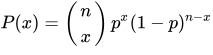
- where p lies between 0 and 1 and n is the number of trials.
Algorithm: acceptance-rejection method BTPEC (Kachitvichyanukul and Schmeiser, 1988).
Poisson
The density function of the Poisson distribution is given by:
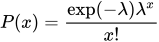
- where parameter λ is greater than zero.
Algorithm: acceptance-rejection (Ahrens and Dieter, 1982a).
Chi-square
The density function of the chi-square distribution is given by:

The deviates are calculated as gamma deviates with parameters n/2 and 2, where n is degrees of freedom.
Algorithm: Transformed gamma deviates (Ahrens and Dieter, 1974,1982b; Gentle 2003).
F (variance ratio)
The density function of the F distribution is given by:

The deviates are calculated as (x/n)/(z/d) where n is the numerator degrees of freedom, d is the denominator degrees of freedom, x is a gamma deviate with parameters n/2 and 2 (chi-square with n degrees of freedom), and z is a gamma deviate with parameters d/2 and 2 (chi-square with d degrees of freedom).
Algorithm: Transformed gamma deviates (Ahrens and Dieter, 1974, 1982b; Gentle 2003).
Student's t
The density function of Student's t distribution is given by:

The deviates are calculated as a standard normal deviate multiplied by the square root of the degrees of freedom (n) divided by a gamma deviate with parameters n/2 and 2 (a chi-square deviate with n degrees of freedom).
Algorithm: Transformed standard normal and gamma deviates (Ahrens and Dieter, 1974, 1982b; Gentle 2003).
Beta
The density function of the beta distribution is given by:
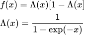
- where a and b are the two shape parameters.
Algorithm: Acceptance-rejection methods BB and BC (Cheng 1978).
Logistic
The density function of the standard logistic distribution is given by:

The deviates are calculated as location + scale * ln(u/(1-u)), where u is a uniform deviate.
Algorithm: Transformed uniform deviates (Gentle 2003).
Cauchy
Algorithm: Transformed uniform deviates (Gentle 2003).
Weibull
Algorithm: Transformed uniform deviates (Gentle 2003).
Geometric
Algorithm: Transformed Poisson and exponential deviates (Devroye, 1986; Gentle 2003; Ahrens and Dieter, 1972, 1982a).
Negative binomial
Algorithm: Transformed Poisson and gamma deviates (Devroye, 1986; Gentle 2003; Ahrens and Dieter, 1974, 1982b, 1982a).
Example
To fill a column with ten random numbers from the standard normal distribution, select Normal from the Random Numbers section of the Generating section of the Data menu. Enter 1 as the number of columns to fill and 10 as the number of rows, keep the population mean of 0 and the population standard deviation of 1, and enter 1234 as the seed in place of the one suggested.
StatsDirect puts these ten numbers (shown here to six decimal places) into a new column of the worksheet, under the heading:
Normal (seed 1234, mean = 0, sd = 1)
-0.872311
0.311024
-0.156733
0.790419
0.772112
-0.604991
-0.593378
0.848327
1.729491
1.154892
The ten values have mean 0.337885 and standard deviation 0.864366: a sample this small from a normal distribution with mean 0 and standard deviation 1 need not look like one. Running the function again with seed 1234 gives the same ten numbers, and any other seed gives a different series. The seed used is always in the column heading, so a series can be repeated even when you accept the seed that StatsDirect suggests.

 R code
This R code reproduces the illustration above in its structure: R's random number generator gives a different series for the same seed. It needs no packages and was checked with R 4.6.1. Paste it into R, or save it as a script and run it.
# Random numbers by distribution: the StatsDirect help illustration (ten standard
# normal deviates from seed 1234, then samples from the other distributions that the
# Data_Generating_Random Numbers menu offers) in R
# StatsDirect and R both use the Mersenne Twister generator, but each seeds it in
# its own way, so the same seed gives a different series in each program. Within one
# program a seed always repeats its own series: set.seed() then the r* function.
set.seed(1234)
x <- rnorm(10, mean = 0, sd = 1)
cat("Normal (seed 1234, mean = 0, sd = 1), from R's generator:\n")
print(round(x, 6))
cat("Mean of the ten =", round(mean(x), 6), " sd =", round(sd(x), 6), "\n")
print(summary(x))

# The menu's other distributions and R's function for each, with StatsDirect's
# parameter names in the comment; n is the number of rows to fill. R's runif and
# StatsDirect's uniform generator both leave out the end points 0 and 1.
n <- 1000
set.seed(1234)
u01 <- runif(n)                            # Uniform 0 to 1
uab <- runif(n, min = 2, max = 5)          # Uniform A to B, interval type
cnt <- sample(1:6, n, replace = TRUE)      # Uniform A to B, count type: whole numbers
ln <- rlnorm(n, meanlog = 0, sdlog = 1)    # Lognormal: log mean, log sd
bi <- rbinom(n, size = 10, prob = 0.3)     # Binomial: number of trials, probability
po <- rpois(n, lambda = 4)                 # Poisson: mean
ga <- rgamma(n, shape = 2, scale = 3)      # Gamma: A (shape), B (scale, 1/lambda)
ex <- rexp(n, rate = 2)                    # Exponential: rate
ch <- rchisq(n, df = 3)                    # Chi-square: degrees of freedom
fv <- rf(n, df1 = 4, df2 = 10)             # F: numerator, denominator df
st <- rt(n, df = 5)                        # Student's t: degrees of freedom
lo <- rlogis(n, location = 0, scale = 1)   # Logistic: mu, sigma
ge <- rgeom(n, prob = 0.3)                 # Geometric: P (failures before a success)
nb <- rnbinom(n, size = 2, prob = 0.5)     # Negative binomial: N, P (failures before
                                           #   the Nth success)
ca <- rcauchy(n, location = 0, scale = 1)  # Cauchy: L (location), S (scale)
we <- rweibull(n, shape = 1.5, scale = 2)  # Weibull: A (shape), sigma (scale)
be <- rbeta(n, shape1 = 2, shape2 = 5)     # Beta: A, B

# A sample's summary should sit close to the distribution's mean and variance: for
# the gamma distribution A * B and A * B^2, for the lognormal exp(mu + sigma^2 / 2)
# and exp(2 * mu + 2 * sigma^2) - exp(2 * mu + sigma^2), for the Poisson its mean
cat("Uniform 0 to 1 (mean 0.5, variance 1/12):\n")
print(summary(u01))
cat("Sample variance =", round(var(u01), 4), "\n")
cat("Gamma (A = 2, B = 3; mean 6, variance 18):\n")
print(summary(ga))
cat("Sample variance =", round(var(ga), 4), "\n")
cat("Lognormal (log mean 0, log sd 1; mean", round(exp(0.5), 4), "variance",
    paste0(round(exp(2) - exp(1), 4), "):"), "\n")
print(summary(ln))
cat("Sample variance =", round(var(ln), 4), "\n")
cat("Poisson (mean 4, variance 4):\n")
print(summary(po))
cat("Sample variance =", round(var(po), 4), "\n")
cat("Binomial (10 trials, p = 0.3; mean 3, variance 2.1):\n")
print(summary(bi))
cat("Sample variance =", round(var(bi), 4), "\n")

# The gamma sample against its density
hist(ga, freq = FALSE, breaks = 30, main = "Gamma (A = 2, B = 3)", xlab = "x")
curve(dgamma(x, shape = 2, scale = 3), add = TRUE, col = "red")