Chi-square Distribution
Menu location: Analysis_Distributions_Chi-Square.
A variable from a chi-square distribution with n degrees of freedom is the sum of the squares of n independent standard normal variables (z).

[chi (Greek χ) is pronounced ki as in kind]
A chi-square variable with one degree of freedom is equal to the square of the standard normal variable. A chi-square variable with many degrees of freedom (n) is approximately normally distributed with mean n and variance 2n, as the central limit theorem dictates.
The so called "linear constraint" property of chi-square explains its application in many statistical methods: Suppose we consider one sub-set of all possible outcomes of n random variables (z). The sub-set is defined by a linear constraint:

- where a and k are constants. Here the sum of the squares of z follows a chi-square distribution with n-1 degrees of freedom. If there are m linear constraints then the total degrees of freedom is n-m. The number of linear constraints associated with the design of contingency tables explains the number of degrees of freedom used in contingency table tests (Bland, 2000).
Another important relationship of chi-square is as follows: the sums of squares about the mean for a normal sample of size n will follow the distribution of the population variance times chi-square with n-1 degrees of freedom. As the expected value of chi-square is n-1 here, the sample variance is estimated as the sums of squares about the mean divided by n-1.
Technical Validation
StatsDirect calculates the probability associated with a chi-square random variable with n degrees of freedom, for this a reliable approach to the incomplete gamma integral is used (Shea, 1988). Chi-square quantiles are calculated for n degrees of freedom and a given probability using the Taylor series expansion of Best and Roberts (1975) when P ≤ 0.999998 and P ≥ 0.000002, otherwise a root finding algorithm is applied to the incomplete gamma integral.
StatsDirect agrees fully with all of the double precision reference values quoted by Shea (1988).
Function Definition
The distribution function F(x) of a chi-square random variable x with n degrees of freedom is:

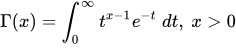
Γ(*) is the gamma function:
Example
Select Chi-Square from the Distributions section of the Analysis menu. Enter a chi-square value and its degrees of freedom, then click Calculate to see the probability in the upper tail of the distribution beyond that value (the P value of a chi-square test). Alternatively enter an upper tail probability and the degrees of freedom, then click Invert to see the chi-square value that cuts off that tail (the critical value for that P).
For example:
P(chi-sq 3.84, df 1) = 0.050043521248705 upper tail
P(chi-sq 15.2, df 6) = 0.018756919725354 upper tail
chi-sq(upper P 0.01, df 3) = 11.3448667301444
A chi-square of 3.84 on one degree of freedom, as from a 2 by 2 table, falls just short of the 5% level, whose critical value is 3.841459; 15.2 on six degrees of freedom, as from a 3 by 4 table, is significant at the 2% level; and a chi-square on three degrees of freedom must exceed 11.3449 to be significant at the 1% level. StatsDirect shows the P to 15 decimal places and the chi-square to 15 significant figures, and writes each result to the report as a probability distribution calculation.

 R code
This R code reproduces the example above. It needs no packages and was checked with R 4.6.1. Paste it into R, or save it as a script and run it.
# Chi-square distribution: the example in the StatsDirect help (the upper tail
# probabilities of two chi-square statistics and the 1% critical value on 3 degrees of
# freedom, as the Distributions dialog computes them) in R
fifteen <- function(x) formatC(x, digits = 15, format = "f", drop0trailing = TRUE)

# The upper tail probability of a chi-square statistic, the P value of a chi-square
# test: pchisq with lower.tail = FALSE (pchisq(x, df) gives the lower tail; subtracting
# that from 1 would lose accuracy far into the upper tail)
cat("P(chi-sq 3.84, df 1) =", fifteen(pchisq(3.84, 1, lower.tail = FALSE)),
    "upper tail\n")
cat("P(chi-sq 15.2, df 6) =", fifteen(pchisq(15.2, 6, lower.tail = FALSE)),
    "upper tail\n")

# With one degree of freedom chi-square is the square of a standard normal deviate, so
# its upper tail is the two sided normal tail beyond the square root of the statistic
cat("Two sided normal P beyond sqrt(3.84) =", fifteen(2 * pnorm(-sqrt(3.84))), "\n")

# The chi-square value that cuts off a given upper tail (the critical value for a P):
# qchisq. StatsDirect shows it to at most 15 decimal places and 15 significant figures
# (13 decimal places for a value above 10), so it is printed the same way here
x15 <- function(x) formatC(x, digits = 15, format = "g", drop0trailing = TRUE)
cat("chi-sq(upper P 0.01, df 3) =", x15(qchisq(0.01, 3, lower.tail = FALSE)), "\n")