Poisson Distribution
Menu location: Analysis_Distributions_Poisson.
A Poisson distribution is the distribution of the number of events in a fixed time interval, provided that the events occur at random, independently in time and at a constant rate.
The event rate, µ, is the number of events per unit time. When µ is large, the shape of a Poisson distribution is very similar to that of the standard normal distribution. The change in shape of a Poisson distribution with increasing n is very similar to the equivalent binomial distribution. Convergence of distributions in this way can be explained by the central limit theorem.
Consider a time interval divided into many sub-intervals of equal length such that the probability of an event in a sub-interval is small and the probability of more than one event is negligible. If the probability of an event in each sub-interval is the same as and independent of that probability for other sub-intervals then n sub-intervals can be thought of as n independent trials. This is why Poisson distributions are closely related to binomial distributions.
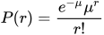
Both the mean and variance of a Poisson distribution are equal to µ. The probability of r events happening in unit time with an event rate of µ is:
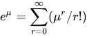
The summation of this Poisson frequency function from zero to r will always be equal to one as:
Analysis of mortality statistics often employs Poisson distributions on the assumption that deaths from most diseases occur independently and at random in populations (see Poisson rate confidence interval). Other common uses of Poisson are in Physics to model radioactive particle emission and in insurance companies to model accident rates.
Technical Validation
StatsDirect calculates cumulative probabilities that (≤,≥,=) r random events are contained in an interval when the average number of such events per interval is μ. The gamma function is a generalised factorial function and it is used to calculate each Poisson probability (Knusel, 1986). The core algorithm evaluates the logarithm of the gamma function (Cody and Hillstrom, 1967; Abramowitz and Stegun 1972; Macleod, 1989) to the limit of 64-bit precision. The inverse is found using a bisection algorithm to one order of magnitude larger than the limit of 64-bit precision.
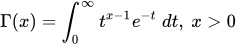
Γ(*) is the gamma function:
Γ(1)=1
Γ(x+1)=xΓ(x)
Γ(n)=(n-1)!
Example
An illustration with invented figures. Suppose that deaths from a cause in a district have averaged 8 a year, and that 14 were recorded in the latest year. If the deaths occur independently and at random at a constant rate, the number in a year follows a Poisson distribution with mean 8.
To calculate the probabilities in StatsDirect select Poisson from the Distributions section of the Analysis menu, enter 14 as the number of random events and 8 as the mean, then click Calculate.
For this example StatsDirect shows the probability of exactly 14 events, of 14 or more and of 14 or fewer, and reports the three on one line:
P(Poisson n 14, µ 8) = 0.016923711395853 for n events, 0.034180701793819 for n or more events, 0.982743009602034 for n or fewer events
These are the exact values to 15 decimal places.
So 14 or more deaths would be seen in about 3.4% of years if the underlying rate had not changed: unusual, but not so rare that a rise in the rate can be inferred from one year alone.
The function also works in reverse: enter a probability in the "or more" or the "or fewer" box and click Invert, and StatsDirect finds the mean that gives that probability for the number of events entered. The Lower CL and Upper CL buttons do this for the two tail probabilities of the confidence level in the box beside them. With 14 events and 95%, the mean at which 14 or more events has probability 0.025 is shown as 7.6539302763006 and the mean at which 14 or fewer events has probability 0.025 as 23.4896211218356 (a mean is shown to 15 significant figures); these are the exact 95% confidence limits for a Poisson count of 14 (see Poisson rate confidence interval).
With a mean of 3 the probability of no events is 0.049787068367864, which is e-3, as the formula above gives for r = 0.
StatsDirect shows a probability to 15 decimal places and a mean to 15 significant figures; the R code below calculates the same figures.

 R code
This R code reproduces the illustration above. It needs no packages and was checked with R 4.6.1. Paste it into R, or save it as a script and run it.
# Poisson distribution: the StatsDirect help illustration (probabilities for a count of
# events with a given mean, and the mean that gives a chosen tail probability) in R

# StatsDirect shows the probabilities of exactly n, of n or more and of n or fewer
# events to 15 decimal places, and a mean to 15 significant figures; these helpers
# print R's values the same way.
p15 <- function(x) formatC(x, digits = 15, format = "f", drop0trailing = TRUE)
s15 <- function(x) trimws(formatC(x, digits = 15, format = "fg", drop0trailing = TRUE))

# 14 events when the mean is 8. dpois(n, mean) is the probability of exactly n events
# and ppois(n, mean) that of n or fewer; with lower.tail = FALSE ppois gives the
# probability of MORE than n events, so the probability of n or more events is
# ppois(n - 1, mean, lower.tail = FALSE)
n <- 14
mu <- 8
cat("Probability of", n, "events =", p15(dpois(n, mu)), "\n")
cat("Probability of", n, "or more events =", p15(ppois(n - 1, mu, lower.tail = FALSE)),
    "\n")
cat("Probability of", n, "or fewer events =", p15(ppois(n, mu)), "\n")

# The inverse: the mean at which n or more events has probability 0.025 and the mean at
# which n or fewer events has probability 0.025 (StatsDirect's Lower CL and Upper CL
# buttons with 95 in the confidence box, found by bisection on the cumulative
# probability). In R they come from the gamma distribution: n or more events with mean
# m has the same probability as the n-th event of a unit-rate process occurring by time
# m, so P(n or more) = pgamma(m, n) and P(n or fewer) = 1 - pgamma(m, n + 1).
lower <- qgamma(0.025, n)
upper <- qgamma(0.975, n + 1)
cat("Mean at which", n, "or more events has probability 0.025 =", s15(lower), "\n")
cat("Mean at which", n, "or fewer events has probability 0.025 =", s15(upper), "\n")
# a check against ppois; these are also the exact 95% limits for a Poisson count of n
cat("  check:", p15(ppois(n - 1, lower, lower.tail = FALSE)), p15(ppois(n, upper)),
    "\n")
cat("  exact 95% confidence interval for a Poisson count of", n, "=", s15(lower), "to",
    s15(upper), "\n")

# No events when the mean is 3: P(0) = exp(-mean)
cat("Probability of 0 events with mean 3 =", p15(dpois(0, 3)), "\n")
cat("  which is exp(-3) =", p15(exp(-3)), "\n")

# R's qpois inverts the other way, for the count: the smallest number of events whose
# probability of that many or fewer is at least the probability given
cat("Smallest count with probability at least 0.95 of that many or fewer, mean 8 =",
    qpois(0.95, mu), "\n")