Log-rank and Wilcoxon

Menu location: Analysis_Survival_Log-rank and Wilcoxon.

This function provides methods for comparing two or more survival curves where some of the observations may be censored and where the overall grouping may be stratified. The methods are nonparametric in that they do not make assumptions about the distributions of survival estimates.

In the absence of censorship (e.g. loss to follow up, alive at end of study) the methods presented here reduce to a Mann-Whitney (two sample Wilcoxon) test for two groups of survival times and a Kruskal-Wallis test for more than two groups of survival times. StatsDirect gives a comprehensive set of tests for the comparison of survival data that may be censored (Tarone and Ware, 1977; Kalbfleisch and Prentice, 1980; Cox and Oakes, 1984; Le, 1997).

The null hypothesis tested here is that the risk of death/event is the same in all groups.

Peto's log-rank test is generally the most appropriate method but the Prentice modified Wilcoxon test is more sensitive when the ratio of hazards is higher at early survival times than at late ones (Peto and Peto, 1972; Kalbfleisch and Prentice, 1980). The log-rank test is similar to the Mantel-Haenszel test and some authors refer to it as the Cox-Mantel test (Mantel and Haenszel, 1959; Cox, 1972).

Strata

An optional variable, strata, allows you to sub-classify the groups specified in the group identifier variable and to test the significance of this sub-classification (Armitage and Berry, 1994; Lawless, 1982; Kalbfleisch and Prentice, 1980).

Wilcoxon weights

StatsDirect gives you a choice of three different weighting methods for the generalised Wilcoxon test, these are Peto-Prentice, Gehan-Breslow and Tarone-Ware. The Peto-Prentice method is generally more robust than the others but the Gehan statistic is calculated routinely by many statistical software packages (Breslow, 1974; Tarone and Ware, 1977; Kalbfleisch and Prentice, 1980; Miller, 1981; Hosmer and Lemeshow 1999). You should seek statistical guidance if you plan to use any weighting method other than Peto-Prentice.

Hazard-ratios

An approximate confidence interval for the log hazard-ratio is calculated using the following estimate of standard error (SE):

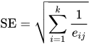
- where e₁ and e₂ are the extents of exposure to risk of death (sometimes called expected deaths) in the two groups compared, each summed over the distinct observed times (Armitage and Berry, 1994).

An exact conditional maximum likelihood estimate of the hazard ratio is also given when there are two groups. The exact estimate and its confidence interval (Fisher or mid-P) should be routinely used in preference to the above approximation. The exponents of Cox regression parameters are also exact estimators of the hazard ratio, but please note that they are not exact if Breslow's method has been used to correct for ties in the regression. Please consult with a statistician if you are considering using Cox regression.

Trend test

If you have more than two groups then StatsDirect will calculate a variant of the log-rank test for trend. If you choose not to enter group scores then they are allocated as 1,2,3 ... n in group order, the order in which the groups first appear in the data and are numbered in the report (Armitage and Berry, 1994; Lawless, 1982; Kalbfleisch and Prentice, 1980).

Technical validation

The general test statistic is calculated around a hypergeometric distribution of the number of events at distinct event times:

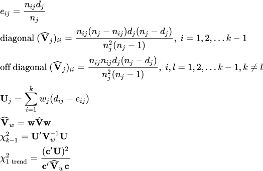
- where the weight w_j for the log-rank test is equal to 1, and w_j for the generalised Wilcoxon test is n_j (Gehan-Breslow method; StatsDirect divides this weight by the number of observations in the stratum plus one, which leaves the chi-square unchanged); for the Tarone-Ware method w_j is the square root of n_j; and for the Peto-Prentice method w_j is a survivor function estimate, the product over the distinct times up to and including the jth of (n_j - d_j + 1) divided by (n_j + 1), which is the weight that SAS uses for the test of Peto and Peto. e_ij is the expectation of death in group i at the jth distinct observed time where d_j events/deaths occurred. n_ij is the number at risk in group i just before the jth distinct observed time, and n_j is the total number at risk at that time. The test statistic for equality of survival across the k groups (populations sampled) is approximately chi-square distributed on k-1 degrees of freedom. The test statistic for monotone trend is approximately chi-square distributed on 1 degree of freedom. c is a vector of scores that are either defined by the user or allocated as 1 to k.

Variance is estimated by the method that Peto (1977) refers to as "exact".

The stratified test statistic is expressed as (Kalbfleisch and Prentice, 1980):

- where the statistics defined above are calculated within strata then summed across strata prior to the generalised inverse and transpose matrix operations.

Example

From Armitage and Berry (1994, p. 479).

Test workbook (Survival worksheet: Stage group, Time, Censor).

The following data represent the survival in days since entry to the trial of patients with diffuse histiocytic lymphoma. Two different groups of patients, those with stage III and those with stage IV disease, are compared.

Stage 3: 6, 19, 32, 42, 42, 43*, 94, 126*, 169*, 207, 211*, 227*, 253, 255*, 270*, 310*, 316*, 335*, 346*

Stage 4: 4, 6, 10, 11, 11, 11, 13, 17, 20, 20, 21, 22, 24, 24, 29, 30, 30, 31, 33, 34, 35, 39, 40, 41*, 43*, 45, 46, 50, 56, 61*, 61*, 63, 68, 82, 85, 88, 89, 90, 93, 104, 110, 134, 137, 160*, 169, 171, 173, 175, 184, 201, 222, 235*, 247*, 260*, 284*, 290*, 291*, 302*, 304*, 341*, 345*

* = censored data (patient still alive or died from an unrelated cause)

To analyse these data in StatsDirect you must first prepare them in three workbook columns as shown below:

Stage group	Time	Censor
1	6	1
1	19	1
1	32	1
1	42	1
1	42	1
1	43	0
1	94	1
1	126	0
1	169	0
1	207	1
1	211	0
1	227	0
1	253	1
1	255	0
1	270	0
1	310	0
1	316	0
1	335	0
1	346	0
2	4	1
2	6	1
2	10	1
2	11	1
2	11	1
2	11	1
2	13	1
2	17	1
2	20	1
2	20	1
2	21	1
2	22	1
2	24	1
2	24	1
2	29	1
2	30	1
2	30	1
2	31	1
2	33	1
2	34	1
2	35	1
2	39	1
2	40	1
2	41	0
2	43	0
2	45	1
2	46	1
2	50	1
2	56	1
2	61	0
2	61	0
2	63	1
2	68	1
2	82	1
2	85	1
2	88	1
2	89	1
2	90	1
2	93	1
2	104	1
2	110	1
2	134	1
2	137	1
2	160	0
2	169	1
2	171	1
2	173	1
2	175	1
2	184	1
2	201	1
2	222	1
2	235	0
2	247	0
2	260	0
2	284	0
2	290	0
2	291	0
2	302	0
2	304	0
2	341	0
2	345	0

Alternatively, open the test workbook using the file open function of the file menu. Then select Log-rank and Wilcoxon from the Survival Analysis section of the analysis menu. Select the column marked "Stage group" when asked for the group identifier, select "Time" when asked for times and "Censor" for censorship. Click on the cancel button when asked about strata.

For this example:

Logrank and Wilcoxon tests

Log-rank (Peto):

For group 1 (Stage group = 1)

Observed deaths = 8

Extent of exposure to risk of death = 16.687031

Relative rate = 0.479414

For group 2 (Stage group = 2)

Observed deaths = 46

Extent of exposure to risk of death = 37.312969

Relative rate = 1.232815

test statistics:

-8.687031, 8.687031

variance-covariance matrix:

11.24706	-11.24706
-11.24706	11.24706

Chi-square for equivalence of death rates = 6.70971 P = 0.0096

Hazard Ratio (approximate 95% confidence interval)

Group 1 vs. Group 2 = 0.388878 (0.218343 to 0.692607)

Conditional maximum likelihood estimates:

Hazard Ratio = 0.381485

Exact Fisher 95% confidence interval = 0.154582 to 0.822411

Exact Fisher one sided P = 0.0051, two sided P = 0.0104

Exact mid-P 95% confidence interval = 0.167398 to 0.783785

Exact mid-P one sided P = 0.0034, two sided P = 0.0068

Generalised Wilcoxon (Peto-Prentice):

test statistics:

-5.185761, 5.185761

variance-covariance matrix:

4.900418	-4.900418
-4.900418	4.900418

Chi-square for equivalence of death rates = 5.487718 P = 0.0192

Both log-rank and Wilcoxon tests demonstrated a statistically significant difference in survival experience between stage 3 and stage 4 patients in this study.

Stratified example

From Peto et al. (1977):

Group	Trial Time	Censorship	Stratum
1	8	1	1
1	8	1	2
2	13	1	1
2	18	1	1
2	23	1	1
1	52	1	1
1	63	1	1
1	63	1	1
2	70	1	2
2	70	1	2
2	180	1	2
2	195	1	2
2	210	1	2
1	220	1	2
1	365	0	2
2	632	1	2
2	700	1	2
1	852	0	2
2	1296	1	2
1	1296	0	2
1	1328	0	2
1	1460	0	2
1	1976	0	2
2	1990	0	2
2	2240	0	2

Censorship 1 = death event

Censorship 0 = lost to follow-up

Stratum 1 = renal impairment

Stratum 2 = no renal impairment

The table above shows you how to prepare data for a stratified log-rank test in StatsDirect. This example is worked through in the second of two classic papers by Richard Peto and colleagues (Peto et al., 1977, 1976). Please note that StatsDirect uses the more accurate variance formulae mentioned in the statistical notes section at the end of Peto et al. (1977).

These data are in the test workbook (Survival worksheet: Group, Trial Time, Censorship, Strat). Select "Group" when asked for the group identifier, "Trial Time" for times, "Censorship" for censorship and "Strat" when asked about strata.

For this example:

Logrank and Wilcoxon tests

Log-rank (Peto) * [STRATUM 1 of 2: Strat=1]:

For group 1 (Group = 1)

Observed deaths = 4

Extent of exposure to risk of death = 5.421429

Relative rate = 0.737813

For group 2 (Group = 2)

Observed deaths = 3

Extent of exposure to risk of death = 1.578571

Relative rate = 1.900452

test statistics:

-1.421429, 1.421429

variance-covariance matrix:

0.922398	-0.922398
-0.922398	0.922398

Chi-square for equivalence of death rates = 2.190442 P = 0.1389

Generalised Wilcoxon (Peto-Prentice) * [STRATUM 1 of 2: Strat=1]:

test statistics:

-0.75, 0.75

variance-covariance matrix:

0.46875	-0.46875
-0.46875	0.46875

Chi-square for equivalence of death rates = 1.2 P = 0.2733

Log-rank (Peto) * [STRATUM 2 of 2: Strat=2]:

For group 1 (Group = 1)

Observed deaths = 2

Extent of exposure to risk of death = 4.98342

Relative rate = 0.401331

For group 2 (Group = 2)

Observed deaths = 8

Extent of exposure to risk of death = 5.01658

Relative rate = 1.594712

test statistics:

-2.98342, 2.98342

variance-covariance matrix:

2.433343	-2.433343
-2.433343	2.433343

Chi-square for equivalence of death rates = 3.657846 P = 0.0558

Log-rank (Peto) for COMBINED STRATA:

Group	Deaths	Extent of exposure to risk of death	Relative rate
1	6	10.404848	0.576654
2	11	6.595152	1.667892

overall chi-square = 5.781939 P = 0.0162

Hazard Ratio (approximate 95% confidence interval)

Group 1 vs. Group 2 = 0.345738 (0.13034 to 0.9171)

Generalised Wilcoxon (Peto-Prentice) * [STRATUM 2 of 2: Strat=2]:

test statistics:

-1.841824, 1.841824

variance-covariance matrix:

1.246236	-1.246236
-1.246236	1.246236

Chi-square for equivalence of death rates = 2.722049 P = 0.099

Generalised Wilcoxon (Peto-Prentice) for COMBINED STRATA:

Group	Deaths	Extent of exposure to risk of death	Relative rate
1	6	10.404848	0.576654
2	11	6.595152	1.667892

overall chi-square = 3.916972 P = 0.0478

Allowing for renal impairment, the death rate differed between the two groups (stratified log-rank test P = 0.0162): the hazard in group 1 was about a third of that in group 2, with a wide confidence interval from so few deaths. Neither stratum alone gave a statistically significant difference.

R code

This R code reproduces the two examples above. It uses the survival package, which comes with R, and was checked with R 4.6.1. Paste it into R, or save it as a script and run it.

# Log-rank and Wilcoxon tests: the StatsDirect help example (Armitage and Berry 1994,
# survival in days of lymphoma patients with stage III or stage IV disease; the test
# workbook's Survival worksheet columns Stage group, Time and Censor) in R
library(survival)
stage <- rep(c(1, 2), c(19, 61))
time <- c(6, 19, 32, 42, 42, 43, 94, 126, 169, 207, 211, 227, 253, 255, 270, 310, 316,
          335, 346, 4, 6, 10, 11, 11, 11, 13, 17, 20, 20, 21, 22, 24, 24, 29, 30, 30,
          31, 33, 34, 35, 39, 40, 41, 43, 45, 46, 50, 56, 61, 61, 63, 68, 82, 85, 88,
          89, 90, 93, 104, 110, 134, 137, 160, 169, 171, 173, 175, 184, 201, 222, 235,
          247, 260, 284, 290, 291, 302, 304, 341, 345)
dead <- c(1, 1, 1, 1, 1, 0, 1, 0, 0, 1, 0, 0, 1, 0, 0, 0, 0, 0, 0, 1, 1, 1, 1, 1, 1, 1,
          1, 1, 1, 1, 1, 1, 1, 1, 1, 1, 1, 1, 1, 1, 1, 1, 0, 0, 1, 1, 1, 1, 0, 0, 1, 1,
          1, 1, 1, 1, 1, 1, 1, 1, 1, 1, 0, 1, 1, 1, 1, 1, 1, 1, 0, 0, 0, 0, 0, 0, 0, 0,
          0, 0)

# R's standard test: the log-rank test. Its Observed and Expected are the report's
# observed deaths and extents of exposure to risk of death, and its chi-square is the
# report's, both using the hypergeometric variance at each death time
print(survdiff(Surv(time, dead) ~ stage))

six <- function(x) formatC(x, digits = 6, format = "f", drop0trailing = TRUE)
pv <- function(p) {
  if (p < 0.0001) "P < 0.0001" else
    paste("P =", formatC(p, digits = 4, format = "f", drop0trailing = TRUE))
}

# The report's statistics from the formulae above, for groups numbered 1 to k. At each
# distinct time the numbers at risk and the deaths in each group give the expected
# deaths, the weighted score U and its variance matrix V. The log-rank weight is 1.
# The Peto-Prentice weight is a survivor function estimate: the product over the
# distinct times up to and including the current time of (n - d + 1) / (n + 1).
# The chi-square drops the last group's row and column, as V is singular.
rank_test <- function(time, dead, group, wilcoxon = FALSE) {
  k <- max(group)
  O <- tabulate(group[dead == 1], k)
  E <- numeric(k)
  U <- numeric(k)
  V <- matrix(0, k, k)
  surv <- 1
  for (t in sort(unique(time))) {
    atrisk <- time >= t
    n <- sum(atrisk)
    ni <- tabulate(group[atrisk], k)
    d <- sum(dead[time == t])
    di <- tabulate(group[time == t & dead == 1], k)
    surv <- surv * (n - d + 1) / (n + 1)
    w <- if (wilcoxon) surv else 1
    E <- E + d * ni / n
    U <- U + w * (di - d * ni / n)
    if (n > 1) {
      V <- V + w^2 * (diag(ni * n, k) - outer(ni, ni)) * d * (n - d) / (n^2 * (n - 1))
    }
  }
  chi <- as.numeric(t(U[-k]) %*% solve(V[-k, -k]) %*% U[-k])
  p <- pchisq(chi, k - 1, lower.tail = FALSE)
  list(O = O, E = E, U = U, V = V, chi = chi, p = p)
}
show_test <- function(r, groups = TRUE) {
  if (groups) {
    for (i in seq_along(r$O)) {
      cat("For group", i, "\n")
      cat("Observed deaths =", r$O[i], "\n")
      cat("Extent of exposure to risk of death =", six(r$E[i]), "\n")
      cat("Relative rate =", six(r$O[i] / r$E[i]), "\n")
    }
  }
  cat("test statistics:", six(r$U), "\n")
  cat("variance-covariance matrix:\n")
  for (i in seq_along(r$O)) cat(six(r$V[i, ]), "\n")
  cat("Chi-square for equivalence of death rates =", six(r$chi), " ", pv(r$p), "\n")
}
cat("Log-rank (Peto):\n")
lr <- rank_test(time, dead, stage)
show_test(lr)

# Hazard ratio: the ratio of the relative rates, with the approximate interval from the
# standard error of its log given above
hazard_ratio <- function(O, E, i, j, level = 0.95) {
  hr <- (O[i] / E[i]) / (O[j] / E[j])
  half <- qnorm((1 + level) / 2) * sqrt(1 / E[i] + 1 / E[j])
  cat("Group ", i, " vs. Group ", j, " = ", six(hr), " (", six(hr * exp(-half)), " to ",
      six(hr * exp(half)), ")\n", sep = "")
}
cat("Hazard Ratio (approximate 95% confidence interval)\n")
hazard_ratio(lr$O, lr$E, 1, 2)

# Conditional maximum likelihood estimate: a 2 by 2 table at each death time (deaths
# and survivors by group among those at risk) and the exact test of a common odds
# ratio across the tables. R's estimate, interval and two sided P agree with the
# report's Fisher figures to five decimal places
death_tables <- function(time, dead, group) {
  cells <- NULL
  for (t in sort(unique(time[dead == 1]))) {
    atrisk <- time >= t
    ni <- tabulate(group[atrisk], 2)
    di <- tabulate(group[time == t & dead == 1], 2)
    if (all(ni > 0)) cells <- c(cells, di, ni - di)
  }
  array(cells, c(2, 2, length(cells) / 4))
}
tables <- death_tables(time, dead, stage)
print(mantelhaen.test(tables, exact = TRUE))

# The same from the conditional distribution of the total deaths in group 1 given the
# margins of every table: the product of the hypergeometric polynomials of the tables,
# scaled as it grows to stay within range. Each side's P counts the observed value in
# full (Fisher) or by half (mid-P); the two sided Fisher P sums the probabilities no
# larger than the observed value's, and the two sided mid-P is twice the smaller side.
# A limit is the ratio at which a tail probability equals half of one minus the level
poly <- 1
low <- 0
for (i in seq_len(dim(tables)[3])) {
  n1 <- sum(tables[1, , i])
  n0 <- sum(tables[2, , i])
  m1 <- sum(tables[, 1, i])
  a <- max(0, m1 - n0):min(m1, n1)
  coef <- choose(n1, a) * choose(n0, m1 - a)
  product <- numeric(length(poly) + length(coef) - 1)
  for (j in seq_along(coef)) {
    at <- j - 1 + seq_along(poly)
    product[at] <- product[at] + poly * coef[j]
  }
  poly <- product / max(product)
  low <- low + a[1]
}
support <- low + seq_along(poly) - 1
A <- sum(tables[1, 1, ])
observed <- which(support == A)
prob <- function(ratio) {
  lp <- log(poly) + (support - low) * log(ratio)
  p <- exp(lp - max(lp))
  p / sum(p)
}
p <- prob(1)
upper <- sum(p[observed:length(p)])
lower <- sum(p[1:observed])
upper_mid <- upper - p[observed] / 2
tail <- function(log_ratio, target, half) {
  q <- prob(exp(log_ratio))
  sum(q[observed:length(q)]) - half * q[observed] - target
}
limit <- function(target, half) {
  exp(uniroot(tail, c(-30, 30), target = target, half = half, tol = 1e-12)$root)
}
mean_deaths <- function(log_ratio) sum(prob(exp(log_ratio)) * support) - A
cmle <- exp(uniroot(mean_deaths, c(-30, 30), tol = 1e-12)$root)
cat("Conditional maximum likelihood estimates:\n")
cat("Hazard Ratio =", six(cmle), "\n")
cat("Exact Fisher 95% confidence interval =", six(limit(0.025, 0)), "to",
    six(limit(0.975, 1)), "\n")
cat("Exact Fisher one sided ", pv(min(upper, lower)), ", two sided ",
    pv(sum(p[p <= p[observed]])), "\n", sep = "")
cat("Exact mid-P 95% confidence interval =", six(limit(0.025, 0.5)), "to",
    six(limit(0.975, 0.5)), "\n")
cat("Exact mid-P one sided ", pv(min(upper_mid, 1 - upper_mid)), ", two sided ",
    pv(min(1, 2 * min(upper_mid, 1 - upper_mid))), "\n", sep = "")

# Generalised Wilcoxon test. R's nearest is the Peto and Peto modification, with the
# Kaplan-Meier estimate as the weight (rho = 1): chi-square 5.45, against the report's
# 5.488 with the Peto-Prentice weight described above
print(survdiff(Surv(time, dead) ~ stage, rho = 1))
cat("Generalised Wilcoxon (Peto-Prentice):\n")
show_test(rank_test(time, dead, stage, wilcoxon = TRUE), groups = FALSE)

# The stratified example (Peto et al. 1977; the test workbook's Survival worksheet
# columns Group, Trial Time, Censorship and Strat): the test within each stratum, then
# the scores and variance matrices summed over the strata for the combined test
trial <- c(8, 8, 13, 18, 23, 52, 63, 63, 70, 70, 180, 195, 210, 220, 365, 632, 700,
           852, 1296, 1296, 1328, 1460, 1976, 1990, 2240)
event <- c(1, 1, 1, 1, 1, 1, 1, 1, 1, 1, 1, 1, 1, 1, 0, 1, 1, 0, 1, 0, 0, 0, 0, 0, 0)
arm <- c(1, 1, 2, 2, 2, 1, 1, 1, 2, 2, 2, 2, 2, 1, 1, 2, 2, 1, 2, 1, 1, 1, 1, 2, 2)
stratum <- c(1, 2, 1, 1, 1, 1, 1, 1, 2, 2, 2, 2, 2, 2, 2, 2, 2, 2, 2, 2, 2, 2, 2, 2, 2)
print(survdiff(Surv(trial, event) ~ arm + strata(stratum)))
combined <- function(wilcoxon) {
  total <- NULL
  for (s in 1:2) {
    r <- rank_test(trial[stratum == s], event[stratum == s], arm[stratum == s],
                   wilcoxon)
    cat("STRATUM", s, "of 2\n")
    show_test(r, groups = !wilcoxon)
    total <- if (is.null(total)) r else Map("+", total, r)
  }
  cat("COMBINED STRATA: group, deaths, extent of exposure to risk of death,",
      "relative rate\n")
  for (i in 1:2) cat(i, total$O[i], six(total$E[i]), six(total$O[i] / total$E[i]), "\n")
  chi <- total$U[1]^2 / total$V[1, 1]
  cat("overall chi-square =", six(chi), " ", pv(pchisq(chi, 1, lower.tail = FALSE)),
      "\n")
  total
}
cat("Log-rank (Peto), stratified:\n")
total <- combined(wilcoxon = FALSE)
cat("Hazard Ratio (approximate 95% confidence interval)\n")
hazard_ratio(total$O, total$E, 1, 2)
cat("Generalised Wilcoxon (Peto-Prentice), stratified:\n")
total <- combined(wilcoxon = TRUE)

P values