Mantel-Haenszel Test and Odds Ratio Meta-analysis
Menu locations:
Analysis_Chi-square_Mantel Haenszel;
Analysis_Meta-analysis_Odds Ratio.
Case-control studies of dichotomous outcomes (e.g. healed or not healed) can be represented by arranging the observed counts into fourfold (2 by 2) tables. The separation of data into different tables or strata represents a sub-grouping, e.g. into age bands. Stratification of this kind is sometimes used to reduce confounding.
The Mantel-Haenszel method provides a pooled odds ratio across the strata of fourfold tables. Meta-analysis is used to investigate the combination or interaction of a group of independent studies, for example a series of fourfold tables from similar studies conducted at different centres.
This StatsDirect function examines the odds ratio for each stratum (a single fourfold table) and for the group of studies as a whole. Exact methods are used here in addition to conventional approximations.
For a single stratum odds ratio is estimated as follows:
| EXPOSURE: | |||
| Exposed | Non-Exposed | ||
| OUTCOME: | Cases: | a | b |
| Non-cases: | c | d | |
Sample estimate of the odds ratio = (ad)/(bc)
For each table, the observed odds ratio is displayed with an exact confidence interval (Martin and Austin, 1991; Sahai and Khurshid, 1996). With very large numbers these calculations can take an appreciable amount of time. If the ’try exact’ option is not selected then the logit (Woolf) interval is given instead. With tables that are entered on screen (the Mantel-Haenszel function of the chi-square section) the option is asked for with the data, and it is for all of the exact methods of the results: the confidence interval of each table, the conditional maximum likelihood estimate of the pooled odds ratio and the confidence interval of I². Counts that are not whole numbers are rounded to the nearest whole number for the exact methods.
The Mantel-Haenszel method is used to estimate the pooled odds ratio for all strata, assuming a fixed effects model:
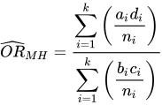
- where ni = ai+bi+ci+di.
Alternative methods, such as Woolf and inverse variance, can be used to estimate the pooled odds ratio with fixed effects but the Mantel-Haenszel method is generally the most robust. A confidence interval for the Mantel-Haenszel odds ratio in StatsDirect is calculated using the Robins, Breslow and Greenland variance formula (Robins et al., 1986) or by the method of Sato (1990) if the estimate of the odds ratio can not be determined. A chi-square test statistic is given with its associated probability that the pooled odds ratio is equal to one; it is calculated from the counts as they are, with a correction of one half for continuity if the difference between the observed and expected numbers of exposed cases, summed over the tables, is one half or more.
If any cell count in a table is zero then a continuity correction is applied to each cell in that table – if you have selected the ’delay continuity correction’ option then no continuity correction is applied to the Mantel-Haenszel calculation unless the product of the ’a’ and ’d’ cells is zero in every study. The type of continuity correction used is set in the options. A table is left out of the pooling, and marked as excluded, if it has no cases in either group, no non-cases in either group, or no subjects in one of the groups.
An exact conditional likelihood method is optionally used to evaluate the pooled odds ratio (Martin and Austin, 2000). The exact method may take an appreciable time to compute with large numbers. The exact results should be used in preference to the Mantel-Haenszel approximation, especially if some categories involve few observations (less than 15 or so).
The inconsistency of results across studies is summarised in the I² statistic, which is the percentage of variation across studies that is due to heterogeneity rather than chance – see the heterogeneity section for more information.
Note that the results from StatsDirect may differ slightly from other software or from those quoted in papers; this is due to differences in the variance formulae. StatsDirect employs the most robust practical approaches to variance according to accepted statistical literature.
DATA INPUT:
Observed frequencies may be entered in a workbook (see example in relative risk meta-analysis) or directly via the screen as multiple fourfold tables:
| feature present | feature absent | |
| outcome positive: | a | b |
| outcome negative: | c | d |
Example
From Armitage and Berry (1994, p. 516).
The following data compare the smoking status of lung cancer patients with controls. Ten different studies are combined in an attempt to improve the overall estimate of relative risk. The matching of controls has been ignored because there was not enough information about matching from each study to be sure that the matching was the same in each study.
| Lung cancer | Controls | ||
| smoker | non-smoker | smoker | non-smoker |
| 83 | 3 | 72 | 14 |
| 90 | 3 | 227 | 43 |
| 129 | 7 | 81 | 19 |
| 412 | 32 | 299 | 131 |
| 1350 | 7 | 1296 | 61 |
| 60 | 3 | 106 | 27 |
| 459 | 18 | 534 | 81 |
| 499 | 19 | 462 | 56 |
| 451 | 39 | 1729 | 636 |
| 260 | 5 | 259 | 28 |
To analyse these data in StatsDirect you may select the Mantel-Haenszel function from the chi-square section of the analysis menu. Select the default 95% confidence interval. Enter the number of tables as 10. Then enter each row of the table above as a separate 2 by 2 contingency table:
i.e. The first row is entered as:
| Smkr | Non | |
| Lung cancer: | 83 | 3 |
| Control: | 72 | 14 |
... this is then repeated for each of the ten rows. Alternatively, open the test workbook, select the odds ratio function from the meta-analysis section of the analysis menu, and select the Meta-analysis worksheet columns "Smokers total", "Smokers cancer", "Control total" and "Control cancer" when prompted for the experimental (smokers) and control (non-smokers) totals and numbers with lung cancer.
For this example:
Fixed effects (Mantel-Haenszel, Robins-Breslow-Greenland)
Pooled odds ratio = 4.681639 (95% CI = 3.865935 to 5.669455)
Chi² (test odds ratio differs from 1) = 292.379352 P < 0.0001
Fixed effects (conditional maximum likelihood)
Pooled odds ratio = 4.713244
Exact Fisher 95% CI = 3.888241 to 5.747141
Exact Fisher one sided P < 0.0001, two sided P < 0.0001
Exact mid-P 95% CI = 3.904839 to 5.719768
Exact mid-P one sided P < 0.0001, two sided P < 0.0001
Non-combinability of studies
Breslow-Day = 6.766765 (df = 9) P = 0.6614
Cochran Q = 6.641235 (df = 9) P = 0.6744
Moment-based estimate of between studies variance = 0
I² (inconsistency) = 0% (95% CI = 0% to 51.7%)
Random effects (DerSimonian-Laird)
Pooled odds ratio = 4.625084 (95% CI = 3.821652 to 5.597423)
Chi² (test odds ratio differs from 1) = 247.466729 (df = 1) P < 0.0001
Bias indicators
Begg-Mazumdar: Kendall's tau = 0.111111 P = 0.7275 (low power)
Egger: bias = 0.580646 (90% CI = -0.6025 to 1.763792) P = 0.3881
Harbord-Egger: bias = 0.792634 (90% CI = -0.56532 to 2.150587) P = 0.3094
Here we can say with 95% confidence that the true population odds in favour of being a smoker were between 3.9 and 5.7 times greater in patients who had lung cancer compared with controls.

 R code
This R code reproduces the example above. It needs no packages and was checked with R 4.6.1. Paste it into R, or save it as a script and run it.
# Odds ratio meta-analysis (Mantel-Haenszel and exact): the StatsDirect help example
# (Armitage and Berry 1994, smoking among lung cancer patients and controls in ten
# case-control studies; the test workbook's Meta-analysis worksheet columns Smokers
# total, Smokers cancer, Control total and Control cancer) in R
smokers <- c(155, 317, 210, 711, 2646, 166, 993, 961, 2180, 519)
smokers_cancer <- c(83, 90, 129, 412, 1350, 60, 459, 499, 451, 260)
nonsmokers <- c(17, 46, 26, 163, 68, 30, 99, 75, 675, 33)
nonsmokers_cancer <- c(3, 3, 7, 32, 7, 3, 18, 19, 39, 5)
k <- length(smokers)

# Each study's fourfold table: a and b are the smokers and non-smokers with lung
# cancer, c and d the smokers and non-smokers among the controls (the workbook's
# "Control" columns are the non-smokers), so the odds ratio a d / (b c) is the odds
# of smoking among the patients relative to the controls
a <- smokers_cancer
b <- nonsmokers_cancer
c <- smokers - a
d <- nonsmokers - b
n <- a + b + c + d
tables <- array(rbind(a, b, c, d), dim = c(2, 2, k),
                dimnames = list(smoking = c("smoker", "non-smoker"),
                                group = c("lung cancer", "control"), study = 1:k))

# R's standard test: the Mantel-Haenszel estimate of the common odds ratio with a
# confidence interval that equals the report's Robins, Breslow and Greenland
# interval, and the Mantel-Haenszel chi-square with the continuity correction
# (correct = TRUE is the default)
r <- mantelhaen.test(tables)
print(r)

# The exact conditional test gives the conditional maximum likelihood estimate and
# the exact (Fisher) interval; R finds them numerically and they agree with the
# report to four significant figures. The code below finds them to a tighter
# tolerance, together with the mid-P interval and P values that R does not print
e <- mantelhaen.test(tables, exact = TRUE)
print(e)

# The report's lines to 6 places
six <- function(x) formatC(x, digits = 6, format = "f", drop0trailing = TRUE)
pv <- function(p) {
  if (p < 0.0001) "P < 0.0001" else
    paste("P =", formatC(p, digits = 4, format = "f", drop0trailing = TRUE))
}
z <- qnorm(0.975)

# The exact methods condition on every table's margins: given them, the total of
# the a cells has a distribution proportional to a product of hypergeometric terms
# times psi^a, where psi is the common odds ratio. The function returns the log of
# each term at psi = 1 over the support of the total (the terms are convolved on the
# natural scale, each table's rescaled to a maximum of 1 to keep within range)
conditional <- function(a, b, c, d) {
  exposed <- a + c
  unexposed <- b + d
  cases <- a + b
  coef <- 1
  start <- 0
  for (i in seq_along(a)) {
    x <- max(0, cases[i] - unexposed[i]):min(exposed[i], cases[i])
    p <- dhyper(x, exposed[i], unexposed[i], cases[i])
    p <- p / max(p)
    new <- numeric(length(coef) + length(p) - 1)
    for (j in seq_along(p)) {
      at <- j:(j + length(coef) - 1)
      new[at] <- new[at] + coef * p[j]
    }
    coef <- new / max(new)
    start <- start + x[1]
  }
  list(support = start + seq_along(coef) - 1, logc = log(coef))
}
# The probability of the part of the support that 'which' selects, at odds ratio psi
cond_p <- function(dist, psi, which) {
  lw <- dist$logc + dist$support * log(psi)
  w <- exp(lw - max(lw))
  sum(w[which]) / sum(w)
}
# Solve for psi on the log scale: the conditional mean equal to the observed total
# (the conditional maximum likelihood estimate), or a tail probability equal to
# alpha / 2 (an exact limit); 'half' counts half of the observed total's probability
# for the mid-P limits
cond_solve <- function(dist, target, s, side = "mean", half = FALSE) {
  f <- function(t) {
    if (side == "mean") {
      lw <- dist$logc + dist$support * t
      w <- exp(lw - max(lw))
      return(sum(dist$support * w) / sum(w) - s)
    }
    p <- if (side == "upper") cond_p(dist, exp(t), dist$support > s) else
      cond_p(dist, exp(t), dist$support < s)
    if (half) p + 0.5 * cond_p(dist, exp(t), dist$support == s) - target else
      p + cond_p(dist, exp(t), dist$support == s) - target
  }
  exp(uniroot(f, c(-30, 30), tol = 1e-10)$root)
}
exact_limits <- function(dist, s, level = 0.95, half = FALSE) {
  alpha <- (1 - level) / 2
  if (s == min(dist$support)) lower <- 0 else
    lower <- cond_solve(dist, alpha, s, "upper", half)
  if (s == max(dist$support)) upper <- Inf else
    upper <- cond_solve(dist, alpha, s, "lower", half)
  c(lower, upper)
}

# Each study's odds ratio with its exact (conditional maximum likelihood) limits,
# as fisher.test would give them, but to a tight tolerance. The report gives the odds
# ratio of a table with an empty cell after a continuity correction, and the exact
# limits of the table as it is; no table has an empty cell here
or <- a * d / (b * c)
lci <- numeric(k)
uci <- numeric(k)
for (i in 1:k) {
  lim <- exact_limits(conditional(a[i], b[i], c[i], d[i]), a[i])
  lci[i] <- lim[1]
  uci[i] <- lim[2]
}
cat("Stratum, odds ratio, 95% CI (CML)\n")
for (i in 1:k) {
  cat(i, six(or[i]), six(lci[i]), six(uci[i]), "\n")
}

# Mantel-Haenszel: the pooled odds ratio is sum(a d / n) / sum(b c / n), the
# fixed effects weights are b c / n, and the Robins-Breslow-Greenland variance of
# its log gives the interval, as mantelhaen.test printed
R <- a * d / n
S <- b * c / n
P <- (a + d) / n
Q <- (b + c) / n
or_mh <- sum(R) / sum(S)
v_rbg <- sum(P * R) / (2 * sum(R)^2) + sum(Q * R + P * S) / (2 * sum(R) * sum(S)) +
  sum(Q * S) / (2 * sum(S)^2)
wt_fixed <- 100 * S / sum(S)

# Heterogeneity: Breslow-Day compares each a cell with its expectation under the
# pooled odds ratio (the root of a quadratic), and Cochran's Q is the weighted sum
# of squared deviations of the log odds ratios from the log of the pooled odds
# ratio, weighted by the inverse of each study's logit (Woolf) variance
cases <- a + b
controls <- c + d
exposed <- a + c
unexposed <- b + d
qa <- 1 - or_mh
qb <- unexposed - cases + (exposed + cases) * or_mh
qc <- -cases * exposed * or_mh
ea <- (-qb + sqrt(qb^2 - 4 * qa * qc)) / (2 * qa)
v_ea <- 1 / (1 / ea + 1 / (cases - ea) + 1 / (exposed - ea) +
               1 / (controls - exposed + ea))
bd <- sum((a - ea)^2 / v_ea)
yi <- log(or)
v_woolf <- 1 / a + 1 / b + 1 / c + 1 / d
w <- 1 / v_woolf
q <- sum(w * (yi - log(or_mh))^2)

# DerSimonian-Laird: the moment estimate of the between studies variance (not less
# than zero), the random effects weights and the pooled odds ratio
tau2 <- max(0, (q - (k - 1)) * sum(w) / (sum(w)^2 - sum(w^2)))
w_re <- 1 / (tau2 + v_woolf)
wt_random <- 100 * w_re / sum(w_re)
or_re <- exp(sum(w_re * yi) / sum(w_re))
x2_re <- sum(w_re * yi)^2 / sum(w_re)

# The report's second table: the standardised effect is the log odds ratio, with
# its logit (Woolf) variance, and the weights are percentages
vi <- v_woolf
cat("Stratum, standardized effect, variance, % weights (fixed, random)\n")
for (i in 1:k) {
  cat(i, six(yi[i]), six(vi[i]), six(wt_fixed[i]), six(wt_random[i]), "\n")
}

mh_ci <- exp(log(or_mh) + c(-1, 1) * z * sqrt(v_rbg))
cat("Fixed effects (Mantel-Haenszel, Robins-Breslow-Greenland)\n")
cat("Pooled odds ratio = ", six(or_mh), " (95% CI = ", six(mh_ci[1]), " to ",
    six(mh_ci[2]), ")\n", sep = "")
x2 <- as.numeric(r$statistic)
cat("Chi2 (test odds ratio differs from 1) =", six(x2), " ", pv(r$p.value), "\n")

# The pooled exact analysis: the conditional maximum likelihood estimate, the exact
# Fisher and mid-P limits, and the P values at odds ratio 1 (the Fisher two sided P
# sums the probabilities of totals no more probable than the one observed)
all <- conditional(a, b, c, d)
s <- sum(a)
cml <- cond_solve(all, 0, s)
fisher <- exact_limits(all, s)
midp <- exact_limits(all, s, half = TRUE)
p_upper <- cond_p(all, 1, all$support >= s)
p_lower <- cond_p(all, 1, all$support <= s)
p_at_s <- cond_p(all, 1, all$support == s)
w1 <- exp(all$logc - max(all$logc))
p2_fisher <- sum(w1[w1 <= w1[all$support == s]]) / sum(w1)
p1_mid <- min(p_upper - p_at_s / 2, 1 - (p_upper - p_at_s / 2))
cat("Fixed effects (conditional maximum likelihood)\n")
cat("Pooled odds ratio =", six(cml), "\n")
cat("Exact Fisher 95% CI =", six(fisher[1]), "to", six(fisher[2]), "\n")
cat("Exact Fisher one sided ", pv(min(p_upper, p_lower)), ", two sided ",
    pv(p2_fisher), "\n", sep = "")
cat("Exact mid-P 95% CI =", six(midp[1]), "to", six(midp[2]), "\n")
cat("Exact mid-P one sided ", pv(p1_mid), ", two sided ", pv(min(1, 2 * p1_mid)),
    "\n", sep = "")

# I-squared is 100 (Q - df) / Q, not below zero. Its interval is the non-central
# chi-square method of Hedges and Pigott (2001) that the report uses: Q is treated
# as a non-central chi-square variable on df degrees of freedom, and each limit is
# the non-centrality parameter at which the observed Q sits at the 97.5th (lower
# limit) or the 2.5th (upper limit) percentile, found with uniroot and pchisq; a
# limit is 0 when the central distribution already puts Q below that percentile.
# A non-centrality lambda gives I-squared = lambda / (df + lambda)
df <- k - 1
isq <- max(0, 100 * (q - df) / q)
ncp_limit <- function(p) {
  if (pchisq(q, df) <= p) return(0)
  # the bracket Q + 1000 is ample: the distribution function there is near 0
  uniroot(function(l) pchisq(q, df, ncp = l) - p, c(0, q + 1000), tol = 1e-10)$root
}
lambda <- c(ncp_limit(0.975), ncp_limit(0.025))
i2_ci <- 100 * lambda / (df + lambda)
one <- function(x) formatC(x, digits = 1, format = "f", drop0trailing = TRUE)
cat("Non-combinability of studies\n")
cat("Breslow-Day = ", six(bd), "  (df = ", df, ")  ",
    pv(pchisq(bd, df, lower.tail = FALSE)), "\n", sep = "")
cat("Cochran Q = ", six(q), "  (df = ", df, ")  ",
    pv(pchisq(q, df, lower.tail = FALSE)), "\n", sep = "")
cat("Moment-based estimate of between studies variance =", six(tau2), "\n")
cat("I2 (inconsistency) = ", one(isq), "% (95% CI = ", one(i2_ci[1]), "% to ",
    one(i2_ci[2]), "%)\n", sep = "")

re_ci <- exp(log(or_re) + c(-1, 1) * z / sqrt(sum(w_re)))
cat("Random effects (DerSimonian-Laird)\n")
cat("Pooled odds ratio = ", six(or_re), " (95% CI = ", six(re_ci[1]), " to ",
    six(re_ci[2]), ")\n", sep = "")
cat("Chi2 (test odds ratio differs from 1) =", six(x2_re), " (df = 1) ",
    pv(pchisq(x2_re, 1, lower.tail = FALSE)), "\n")

# Bias indicators, from the log odds ratios and their logit standard errors.
# Begg-Mazumdar: Kendall's tau between the deviations of the log odds ratios from
# their weighted mean, standardised, and the variances; cor.test gives the exact
# two sided P because there are fewer than 50 studies and no ties. With tied
# variances the report uses tau-b and a continuity-corrected normal approximation,
# cor.test(..., exact = FALSE, continuity = TRUE). The report adds "(low power)"
# with fewer than eleven studies: the rank correlation test then has little power
se <- sqrt(v_woolf)
dev <- (yi - sum(w * yi) / sum(w)) / sqrt(v_woolf - 1 / sum(w))
begg <- cor.test(dev, v_woolf, method = "kendall")
cat("Bias indicators\n")
cat("Begg-Mazumdar: Kendall's tau =", six(begg$estimate), " ", pv(begg$p.value),
    "(low power)\n")
# Egger: the standardised effect regressed on precision, the intercept being the
# bias; the limits are at 90% (twice the usual alpha) because the test has low power
egger <- lm(I(yi / se) ~ I(1 / se))
ci <- confint(egger, level = 0.9)
cat("Egger: bias = ", six(coef(egger)[1]), " (90% CI = ", six(ci[1, 1]),
    " to ", six(ci[1, 2]), ")  ", pv(summary(egger)$coefficients[1, 4]), "\n", sep = "")
# Harbord-Egger: the same regression of each study's efficient score (a minus its
# expectation) divided by the root of its hypergeometric variance, on that root
score <- a - cases * exposed / n
v_score <- cases * controls * exposed * unexposed / (n^2 * (n - 1))
harbord <- lm(I(score / sqrt(v_score)) ~ sqrt(v_score))
ci <- confint(harbord, level = 0.9)
cat("Harbord-Egger: bias = ", six(coef(harbord)[1]), " (90% CI = ",
    six(ci[1, 1]), " to ", six(ci[1, 2]), ")  ",
    pv(summary(harbord)$coefficients[1, 4]), "\n", sep = "")

# The report's charts. First the bias assessment (funnel) plot: each log odds ratio
# against its logit standard error, the axis reversed so that the 95% cone about the
# pooled Mantel-Haenszel log odds ratio opens downwards
se_top <- max(se) * 1.05
plot(yi, se, ylim = c(se_top, 0), xlab = "Log(Odds ratio)", ylab = "Standard error",
     main = "Bias assessment plot",
     xlim = range(yi, log(or_mh) + c(-1, 1) * z * se_top))
abline(v = log(or_mh))
lines(log(or_mh) + c(-1, 0, 1) * z * se_top, c(se_top, 0, se_top))

# The L'Abbe plot: the percentage of each study's smokers who were lung cancer
# patients against the same percentage of its non-smokers, the symbol size growing
# with the study size, with the line of equality. The report adds a dashed line from
# the origin with the slope of the pooled odds ratio, which is the line of a risk
# ratio; the curve of the studies that share the pooled odds ratio is drawn here
p0 <- 100 * b / (b + d)
p1 <- 100 * a / (a + c)
plot(p0, p1, xlim = c(0, 100), ylim = c(0, 100), cex = 0.5 + 2 * sqrt(n / max(n)),
     xlab = "control percent", ylab = "experimental percent",
     main = "L'Abbe plot (symbol size represents sample size)")
abline(0, 1)
x0 <- seq(0, 1, 0.01)
lines(100 * x0, 100 * or_mh * x0 / (1 + (or_mh - 1) * x0), lty = 2)

# The two forest plots: each study's odds ratio (the symbol area proportional to
# its weight) with its exact interval on a log scale, the line of no effect at 1,
# and the pooled estimate as a diamond at the foot with a dashed line up from it
forest <- function(pooled, lower, upper, weights, main, label) {
  y <- (k + 1):2
  two <- function(x) formatC(x, digits = 2, format = "f")
  par(mar = c(5, 8, 4, 9))
  plot(NA, xlim = range(1, lci, uci, lower, upper), ylim = c(0.5, k + 1.5),
       log = "x", yaxt = "n", xlab = "odds ratio (95% confidence interval)",
       ylab = "", main = main)
  abline(v = 1)
  segments(pooled, 1, pooled, k + 1, lty = 2)
  segments(lci, y, uci, y)
  points(or, y, pch = 15, cex = 0.5 + 2 * sqrt(weights / max(weights)))
  polygon(c(lower, pooled, upper, pooled), c(1, 1.3, 1, 0.7), col = "grey")
  axis(2, at = c(y, 1), labels = c(paste("stratum", 1:k), label), las = 1,
       tick = FALSE)
  axis(4, at = c(y, 1), tick = FALSE, las = 1,
       labels = paste0(two(c(or, pooled)), " (", two(c(lci, lower)), ", ",
                       two(c(uci, upper)), ")"))
}
forest(or_mh, mh_ci[1], mh_ci[2], wt_fixed,
       "Odds ratio meta-analysis plot [fixed effects]", "combined [fixed]")
forest(or_re, re_ci[1], re_ci[2], wt_random,
       "Odds ratio meta-analysis plot [random effects]", "combined [random]")
par(mar = c(5, 4, 4, 2) + 0.1)