Proportion Meta-analysis
Menu location: Analysis_Meta-Analysis_Proportion.
This function enables you to calculate an overall proportion from a set of proportions, for example from a systematic review of studies of adherence with a particular drug treatment.
This function can also be applied to a review of diagnostic test studies to give an overall sensitivity or specificity as follows:
| DISEASE/OUTCOME | |||
| Present | Absent | ||
| TEST: | +: | a (true +ve) | b (false +ve) |
| -: | c (false -ve) | d (true -ve) | |
Sensitivity = a/(a+c)
Specificity = d/(b+d)
Another way to summarise diagnostic test performance is via the diagnostic odds ratio:
Diagnostic odds ratio = true/false = (a * d)/(b * c)
In order to run a meta-analysis of diagnostic odds ratios simply use the odds ratio meta-analysis function with the experimental group as the true (test correct) outcomes and the control group as the false outcomes – enter a as experimental group responders; a+d as experimental group number; b as control group responders; and b+c as control group total.
Many study designs can be expressed as a proportion, and relatively complex statistical models can be explored using sets of proportions – for example a random effects logistic regression. You should seek the assistance of a statistician if you want to pursue analyses deeper than the summaries that this StatsDirect function offers.
The inconsistency of results across studies is summarised in the I² statistic, which is the percentage of variation across studies that is due to heterogeneity rather than chance – see the heterogeneity section for more information.
Beyond this meta-analysis function, logistic regression can be used to compare pooled proportions. Consult with a statistician if you are considering a random effects logistic model.
DATA INPUT:
You enter the number of subjects responding (with the study outcome) and the total number of subjects studied. You may also enter a title for each study.
Technical Validation
StatsDirect first transforms proportions via the Freeman-Tukey double arcsine method (Freeman and Tukey, 1950, Miller 1978) then performs an inverse-variance weighted fixed and random effects meta-analysis by conventional methods (DerSimonian and Laird, 1986). The appropriate weight is n+0.5 but some other software uses n+1. In our own simulation testing of the variance options within the formula 1/(n+c), varying c from 0.5 to 1, we found that the n+1 method (Stuart and Ord, 1994) is conservative, avoiding underestimation of the true variance of the transformed proportion, but the original n+0.5 method (Freeman et al, 1950) method is closer to the true variance in absolute terms. Note that there is no fixed transformation of a binomial proportion that provides optimal variance stabilization, which depends on your data - iterative variance stabilization methods may emerge with further research. The pooled proportion can be calculated as the back-transform of the weighted mean of the transformed proportions (Miller 1978):





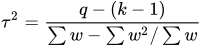
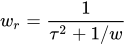
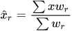

- where p hat is the fixed effects pooled proportion, x is the Freeman-Tukey transformed proportion, w is the inverse variance weight for the transformed proportion, q is the Cochran q statistic, tau squared is the moment-based estimate of the between-studies variance, w r is the DerSimonian-Laird weight, p hat r is the random effects estimate of the pooled proportion, and n in the back-transforms to p hat and p hat r is the harmonic mean of the study sample sizes.
An alternative, simpler, back transform (Stuart-Ord), which is the default choice of inverse transform in StatsDirect, is:
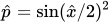
This form is strictly less accurate than the Miller method above but it is less susceptible to the bias effects of non-linear transformations, giving more credible estimates of pooled proportions where the true population value is close to 0 or 1.
Example
The following data represent adherence with medication from 22 fictitious trials of a class of drug:
| Trial | Adherent | Total |
| Brown | 214 | 311 |
| Lamont | 58 | 65 |
| Lally | 59 | 67 |
| Orwell | 182 | 285 |
| Wagner | 65 | 73 |
| Werner | 66 | 116 |
| Venner | 99 | 183 |
| Adams | 600 | 696 |
| Brenner | 45 | 57 |
| Borrowdale | 165 | 277 |
| Byers | 32 | 35 |
| Daniels | 49 | 60 |
| Darling | 175 | 199 |
| Ehert | 155 | 311 |
| Fern | 64 | 81 |
| Mullen | 526 | 537 |
| Orton | 104 | 107 |
| Jones | 97 | 102 |
| Ning | 2310 | 4612 |
| Sherraton | 72 | 91 |
| Zu | 37 | 37 |
| Tarone | 31 | 87 |
To analyse these data in StatsDirect first prepare them in three workbook columns and label these columns appropriately. Alternatively, open the test workbook using the file open function of the file menu. Then select proportion from the meta-analysis section of the analysis menu, and then select the columns 'Total', 'Adherent' and 'Trial' as prompted.
For this example:
Method: Stuart-Ord (inverse double arcsine square root)
| Stratum | Proportion | 95% CI (exact) | ||
| 1 | 0.688103 | 0.633392 | 0.739187 | Brown |
| 2 | 0.892308 | 0.790618 | 0.955591 | Lamont |
| 3 | 0.880597 | 0.778215 | 0.947015 | Lally |
| 4 | 0.638596 | 0.579853 | 0.694424 | Orwell |
| 5 | 0.890411 | 0.795436 | 0.951484 | Wagner |
| 6 | 0.568966 | 0.473763 | 0.660561 | Werner |
| 7 | 0.540984 | 0.465895 | 0.614723 | Venner |
| 8 | 0.862069 | 0.834196 | 0.886827 | Adams |
| 9 | 0.789474 | 0.66113 | 0.88621 | Brenner |
| 10 | 0.595668 | 0.5353 | 0.653966 | Borrowdale |
| 11 | 0.914286 | 0.769425 | 0.981962 | Byers |
| 12 | 0.816667 | 0.695604 | 0.904764 | Daniels |
| 13 | 0.879397 | 0.825884 | 0.921178 | Darling |
| 14 | 0.498392 | 0.441461 | 0.555354 | Ehert |
| 15 | 0.790123 | 0.685373 | 0.872724 | Fern |
| 16 | 0.979516 | 0.963644 | 0.989731 | Mullen |
| 17 | 0.971963 | 0.920245 | 0.99418 | Orton |
| 18 | 0.95098 | 0.889304 | 0.983894 | Jones |
| 19 | 0.500867 | 0.486332 | 0.515402 | Ning |
| 20 | 0.791209 | 0.693308 | 0.869362 | Sherraton |
| 21 | 1 | 0.905109 | 1 | Zu [97.5% one-sided CI] |
| 22 | 0.356322 | 0.256493 | 0.466236 | Tarone |
| Stratum | Standardized effect | Variance | % Weights (fixed, random) | ||
| 1 | 1.955196 | 0.00321 | 3.708333 | 4.657589 | Brown |
| 2 | 2.45427 | 0.015267 | 0.779762 | 4.459405 | Lamont |
| 3 | 2.419139 | 0.014815 | 0.803571 | 4.466536 | Lally |
| 4 | 1.850661 | 0.003503 | 3.39881 | 4.652575 | Orwell |
| 5 | 2.450333 | 0.013605 | 0.875 | 4.485712 | Wagner |
| 6 | 1.707983 | 0.008584 | 1.386905 | 4.56713 | Werner |
| 7 | 1.65241 | 0.00545 | 2.184524 | 4.619459 | Venner |
| 8 | 2.379077 | 0.001436 | 8.291667 | 4.688254 | Adams |
| 9 | 2.176196 | 0.017391 | 0.684524 | 4.426224 | Brenner |
| 10 | 1.762619 | 0.003604 | 3.303571 | 4.650846 | Borrowdale |
| 11 | 2.508913 | 0.028169 | 0.422619 | 4.265199 | Byers |
| 12 | 2.243481 | 0.016529 | 0.720238 | 4.439636 | Daniels |
| 13 | 2.426484 | 0.005013 | 2.375 | 4.626852 | Darling |
| 14 | 1.567591 | 0.00321 | 3.708333 | 4.657589 | Ehert |
| 15 | 2.181244 | 0.01227 | 0.970238 | 4.50708 | Fern |
| 16 | 2.848202 | 0.00186 | 6.39881 | 4.680878 | Mullen |
| 17 | 2.780486 | 0.009302 | 1.279762 | 4.555298 | Orton |
| 18 | 2.675681 | 0.009756 | 1.220238 | 4.547858 | Jones |
| 19 | 1.572531 | 0.000217 | 54.910714 | 4.709554 | Ning |
| 20 | 2.184792 | 0.010929 | 1.089286 | 4.528741 | Sherraton |
| 21 | 2.978651 | 0.026667 | 0.446429 | 4.286939 | Zu [97.5% one-sided CI] |
| 22 | 1.282717 | 0.011429 | 1.041667 | 4.520646 | Tarone |
Fixed effects (inverse variance)
Pooled proportion = 0.63958 (95% CI = 0.629281 to 0.649814)
Non-combinability of studies
Cochran Q = 1553.004499 (df = 21) P < 0.0001
Moment-based estimate of between studies variance = 0.268086
I² (inconsistency) = 98.6% (95% CI = 98.5% to 98.8%)
Random effects (DerSimonian-Laird)
Pooled proportion = 0.785824 (95% CI = 0.689259 to 0.868571)
Bias indicators
Begg-Mazumdar: Kendall's tau = -0.272727 P = 0.0803
Egger: bias = -0.692257 (90% CI = -7.606501 to 6.221986) P = 0.8646
Harbord: bias = 6.349191 (90% CI = 2.914719 to 9.783663) P = 0.0046
The differences between trials are very large (99% inconsistency), therefore a random effects model should be followed. The weights table shows both the fixed and random effects weights – the random effects weights used to calculate the pooled proportion are similar across the studies, unlike the fixed effects weights. We conclude that the adherence for this class of drug is approximately 79%, and with 95% confidence at least 69%. Of the bias indicators, only Harbord's test points to small-study effects: the smaller trials reported higher adherence than the pooled proportion predicts.

 R code
This R code reproduces the example above. It needs no packages and was checked with R 4.6.1. Paste it into R, or save it as a script and run it.
# Proportion meta-analysis: the StatsDirect help example (adherence with medication in
# 22 fictitious trials; the test workbook's Meta-analysis worksheet columns Trial,
# Adherent and Total) in R
trial <- c("Brown", "Lamont", "Lally", "Orwell", "Wagner", "Werner", "Venner", "Adams",
           "Brenner", "Borrowdale", "Byers", "Daniels", "Darling", "Ehert", "Fern",
           "Mullen", "Orton", "Jones", "Ning", "Sherraton", "Zu", "Tarone")
adherent <- c(214, 58, 59, 182, 65, 66, 99, 600, 45, 165, 32, 49, 175, 155, 64, 526,
              104, 97, 2310, 72, 37, 31)
total <- c(311, 65, 67, 285, 73, 116, 183, 696, 57, 277, 35, 60, 199, 311, 81, 537,
           107, 102, 4612, 91, 37, 87)

# Base R has no meta-analysis function, so the pooled proportions are computed as the
# formulae above give them: each proportion is transformed by the Freeman-Tukey double
# arcsine, pooled with inverse variance weights (n + 0.5), and the pooled transform is
# taken back to a proportion by the Stuart-Ord inverse, sin(x/2)^2
six <- function(x) formatC(x, digits = 6, format = "f", drop0trailing = TRUE)
pv <- function(p) {
  if (p < 0.0001) "P < 0.0001" else
    paste("P =", formatC(p, digits = 4, format = "f", drop0trailing = TRUE))
}
k <- length(total)
z <- qnorm(0.975)
p <- adherent / total

# Each study's proportion with its exact (Clopper-Pearson) 95% confidence interval, as
# binom.test() gives it; when every subject responds, as in the Zu trial, the interval
# is one sided and its lower limit is the 97.5% limit
ci <- t(sapply(seq_len(k), function(i) binom.test(adherent[i], total[i])$conf.int))
one_sided <- ifelse(adherent == 0 | adherent == total, "[97.5% one-sided CI]", "")
cat("Method: Stuart-Ord (inverse double arcsine square root)\n")
print(data.frame(Study = seq_len(k), Proportion = six(p), Lower = six(ci[, 1]),
                 Upper = six(ci[, 2]), Trial = paste(trial, one_sided)),
      row.names = FALSE, right = FALSE)

# The transformed proportions, their variances and the fixed and random effects weights
x <- asin(sqrt(adherent / (total + 1))) + asin(sqrt((adherent + 1) / (total + 1)))
v <- 1 / (total + 0.5)
w <- 1 / v
xf <- sum(w * x) / sum(w)
se_f <- 1 / sqrt(sum(w))
q <- sum(w * (x - xf)^2)
tau2 <- max(0, (q - (k - 1)) / (sum(w) - sum(w^2) / sum(w)))
wr <- 1 / (tau2 + v)
xr <- sum(wr * x) / sum(wr)
se_r <- 1 / sqrt(sum(wr))
print(data.frame(Study = seq_len(k), Transform = six(x), Variance = six(v),
                 Fixed = six(100 * w / sum(w)), Random = six(100 * wr / sum(wr)),
                 Trial = paste(trial, one_sided)), row.names = FALSE, right = FALSE)

inv <- function(t) sin(t / 2)^2
cat("Fixed effects (inverse variance)\n")
cat("Pooled proportion = ", six(inv(xf)), " (95% CI = ", six(inv(xf - z * se_f)),
    " to ", six(inv(xf + z * se_f)), ")\n", sep = "")

# Cochran's Q against chi-square on k - 1 df, the DerSimonian-Laird estimate of the
# between-studies variance, and I-squared, which is lambda / (df + lambda) for the
# noncentrality parameter lambda = Q - df, with the confidence interval that StatsDirect
# gives by default (the noncentral chi-square method of Hedges and Pigott): the lambda
# at which the observed Q is the 97.5% point of the noncentral chi-square distribution
# on df degrees of freedom, and the lambda at which it is the 2.5% point, each turned
# into an I-squared; a limit is 0 when the central distribution already puts Q below
# that point
cat("Non-combinability of studies\n")
cat("Cochran Q = ", six(q), "  (df = ", k - 1, ")  ",
    pv(pchisq(q, k - 1, lower.tail = FALSE)), "\n", sep = "")
cat("Moment-based estimate of between studies variance =", six(tau2), "\n")
df <- k - 1
i2 <- function(lambda) 100 * lambda / (df + lambda)
lambda_at <- function(prob) {
  if (pchisq(q, df) < prob) return(0)
  uniroot(function(l) pchisq(q, df, ncp = l) - prob, c(0, 10 * (q + df)),
          tol = 1e-10)$root
}
one <- function(x) formatC(x, digits = 1, format = "f")
cat("I2 (inconsistency) = ", one(i2(max(0, q - df))), "% (95% CI = ",
    one(i2(lambda_at(0.975))), "% to ", one(i2(lambda_at(0.025))), "%)\n", sep = "")

cat("Random effects (DerSimonian-Laird)\n")
cat("Pooled proportion = ", six(inv(xr)), " (95% CI = ", six(inv(xr - z * se_r)),
    " to ", six(inv(xr + z * se_r)), ")\n", sep = "")

# Bias indicators, all on the proportion scale with each study's standard error taken
# from its exact confidence interval. Begg-Mazumdar: Kendall's tau between the
# standardised deviates from the pooled proportion and the variances, with the exact P
# that cor.test() gives when there are no ties. Egger: the intercept of the regression
# of the standardised proportion on precision, with a 90% interval and its t test
cat("Bias indicators\n")
se <- (ci[, 2] - ci[, 1]) / 2 / z
wx <- 1 / se^2
ts <- (p - sum(p * wx) / sum(wx)) / sqrt(se^2 - 1 / sum(wx))
begg <- cor.test(ts, se^2, method = "kendall")
cat("Begg-Mazumdar: Kendall's tau =", six(begg$estimate), " ", pv(begg$p.value), "\n")
egger <- lm(I(p / se) ~ I(1 / se))
cat("Egger: bias = ", six(coef(egger)[1]), " (90% CI = ",
    six(confint(egger, level = 0.9)[1, 1]), " to ",
    six(confint(egger, level = 0.9)[1, 2]), ")  ",
    pv(summary(egger)$coefficients[1, 4]), "\n", sep = "")

# Harbord's test as StatsDirect adapts it to proportions: each study's score is the
# excess of responders over the number expected at the pooled fixed effects proportion,
# with the binomial variance, and the bias is the intercept of the regression of
# score / sqrt(variance) on sqrt(variance)
pf <- inv(xf)
score <- adherent - total * pf
vs <- total * pf * (1 - pf)
harbord <- lm(I(score / sqrt(vs)) ~ sqrt(vs))
cat("Harbord: bias = ", six(coef(harbord)[1]), " (90% CI = ",
    six(confint(harbord, level = 0.9)[1, 1]), " to ",
    six(confint(harbord, level = 0.9)[1, 2]), ")  ",
    pv(summary(harbord)$coefficients[1, 4]), "\n", sep = "")

# The report's charts: a funnel plot of each proportion against its standard error,
# with the pooled fixed effects proportion and its 95% limits, then a forest plot for
# each model with the studies in order from the top and the pooled estimate at the foot
plot(p, se, ylim = rev(c(0, max(se))), xlim = c(0, 1), xlab = "Proportion",
     ylab = "Standard error", main = "Bias assessment plot")
abline(v = pf)
s <- seq(0, max(se), length.out = 50)
lines(pf - z * s, s, lty = 2)
lines(pf + z * s, s, lty = 2)
forest <- function(est, lower, upper, weight, title) {
  rows <- c(trial, "combined")
  y <- rev(seq_along(rows))
  old <- par(mar = c(5, 7, 4, 10))
  plot(est, y, type = "n", xlim = c(0, 1), yaxt = "n", ylab = "",
       xlab = "proportion (95% confidence interval)", main = title)
  segments(lower, y, upper, y)
  points(est[1:k], y[1:k], pch = 15, col = "grey", cex = 3 * sqrt(weight / max(weight)))
  points(est[1:k], y[1:k], pch = 20)
  points(est[k + 1], y[k + 1], pch = 18, cex = 2)
  abline(v = est[k + 1], lty = 3)
  axis(2, at = y, labels = rows, las = 1, tick = FALSE, cex.axis = 0.7)
  axis(4, at = y, tick = FALSE, las = 1, cex.axis = 0.7,
       labels = sprintf("%.2f (%.2f, %.2f)", est, lower, upper))
  par(old)
}
forest(c(p, inv(xf)), c(ci[, 1], inv(xf - z * se_f)), c(ci[, 2], inv(xf + z * se_f)), w,
       "Proportion meta-analysis plot [fixed effects]")
forest(c(p, inv(xr)), c(ci[, 1], inv(xr - z * se_r)), c(ci[, 2], inv(xr + z * se_r)),
       wr, "Proportion meta-analysis plot [random effects]")

# The Miller inverse, the other choice of back-transform in StatsDirect: the exact
# inverse of the double arcsine at n = the harmonic mean of the study sizes
hm <- k / sum(1 / total)
ft <- function(r, n) asin(sqrt(r / (n + 1))) + asin(sqrt((r + 1) / (n + 1)))
miller <- function(t) {
  # beyond the range of the transform at n = hm the exact inverse folds back, so
  # StatsDirect returns 0 or 1 there
  if (t > ft(hm, hm)) return(1)
  if (t < ft(0, hm)) return(0)
  0.5 * (1 - sign(cos(t)) * sqrt(1 - (sin(t) + (sin(t) - 1 / sin(t)) / hm)^2))
}
cat("Method: Miller (exact inverse Freeman-Tukey double arcsine)\n")
cat("Fixed effects pooled proportion = ", six(miller(xf)), " (95% CI = ",
    six(miller(xf - z * se_f)), " to ", six(miller(xf + z * se_f)), ")\n", sep = "")
cat("Random effects pooled proportion = ", six(miller(xr)), " (95% CI = ",
    six(miller(xr - z * se_r)), " to ", six(miller(xr + z * se_r)), ")\n", sep = "")
# Harbord's score is taken from the Miller pooled proportion here, so the test moves
pf <- miller(xf)
score <- adherent - total * pf
vs <- total * pf * (1 - pf)
harbord <- lm(I(score / sqrt(vs)) ~ sqrt(vs))
cat("Harbord: bias = ", six(coef(harbord)[1]), " (90% CI = ",
    six(confint(harbord, level = 0.9)[1, 1]), " to ",
    six(confint(harbord, level = 0.9)[1, 2]), ")  ",
    pv(summary(harbord)$coefficients[1, 4]), "\n", sep = "")