Kendall's Tau Distribution
Menu location: Analysis_Distributions_Kendall's tau.
Given a value for the test statistic (S) associated with Kendall's tau (t) this function calculates the probability of obtaining a value greater than or equal to S for a given sample size.
Consider two samples, x and y, each of size n. The total number of possible pairings of x with y observations is n(n-1)/2. Now consider ordering the pairs by the x values and then by the y values. If x3 > y3 when ordered on both x and y then the third pair is concordant, otherwise the third pair is discordant. S is the difference between the number of concordant (ordered in the same way, nc) and discordant (ordered differently, nd) pairs.
Tau (τ) is related to S by:
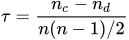
If there are tied (same value) observations then τb is used:

- where ti is the number of observations tied at a particular rank of x and u is the number tied at a rank of y. When there are no ties τb = τ.
This function does not calculate probabilities for τb.
Technical Validation
Probabilities are calculated by summation across all permutations when n ≤ 50 and by an Edgeworth series approximation when n > 50 (Best and Gipps, 1974). The series is within 0.0000005 of the exact probability at n = 51 and within 0.00000003 by n = 100; in the far tail it is less good in proportion to the probability. The two samples are assumed to have been ranked without ties.
The inverse is calculated by finding the largest value of S that gives a calculated upper tail probability (using the method above) closest to but not less than the P value entered. Please note that the results may differ slightly from tables in textbooks because StatsDirect calculates the inverse of Kendall's statistic more accurately than the routines used to calculate Best's widely quoted 1974 table.
Illustration
Consider the ten pairs of rankings in the Kendall rank correlation example, a tutor's rankings of ten students for suitability to their career and for knowledge of psychology. There are 34 concordant and 11 discordant pairs, so S = 23 and τ = 23/45 = 0.511111. To calculate the probability of an S at least this large when the two rankings are independent, select Kendall's tau from the Distributions section of the Analysis menu, enter 10 as the sample size and 23 as S (or enter 0.511111 as tau, from which StatsDirect calculates S) and click Calculate. StatsDirect shows the upper tail probability and reports it as:
P(Kendall's T 23, n 10) = 0.023311287477954 upper tail
Of the 10! = 3,628,800 equally likely orderings of one ranking against the other, 84,592 give an S of 23 or more. This is the upper side P of the exact test in the Kendall rank correlation report (P = 0.0233); the distribution of S is symmetrical about zero, so the two sided P is twice it (P = 0.0466).
For the inverse, enter 10 as the sample size and 0.05 as the upper tail P and click Invert. StatsDirect finds the largest S whose upper tail probability is not less than 0.05, shows it with its tau (S = 19, τ = 0.422222 to six places) and reports the probability that it cuts off:
Kendall's T (upper tail P 0.05, n 10) = 0.054156746031746
So with ten pairs an S of 19 does not quite reach the one sided 5% level. The next possible value, S = 21 (τ = 0.466667), is the smallest that does, with an upper tail probability of 0.036275077160494: with so few pairs the attainable significance levels are coarse.
StatsDirect displays the probabilities in this illustration to 15 decimal places; the R code below reproduces them.

 R code
This R code reproduces the illustration above. It needs no packages and was checked with R 4.6.1. Paste it into R, or save it as a script and run it.
# Kendall's tau distribution: the StatsDirect help illustration (S = 23 for the 10 pairs
# of rankings of the Kendall rank correlation example, Armitage and Berry 1994, p. 466,
# the test workbook's Nonparametric worksheet columns Career and Psychology; and the S
# that cuts off an upper tail of 0.05) in R
career <- c(4, 10, 3, 1, 9, 2, 6, 7, 8, 5)
psychology <- c(5, 8, 6, 2, 10, 3, 9, 4, 7, 1)
n <- length(career)                       # 10 pairs

# For each pair of students, +1 if the two rankings order them the same way (a
# concordant pair), -1 if they order them differently (discordant); S is the sum
q <- sign(outer(career, career, "-")) * sign(outer(psychology, psychology, "-"))
concordant <- sum(q[upper.tri(q)] > 0)
discordant <- sum(q[upper.tri(q)] < 0)
S <- concordant - discordant
cat(concordant, "concordant and", discordant, "discordant pairs, so S =", S, "\n")

# The distribution of S for n pairs ranked without ties when the two rankings are
# independent: each of the n! orderings of one ranking against the other is equally
# likely. For n = 5 all 120 orderings can be listed and S counted for each
perms <- function(m) {
  if (m == 1) return(matrix(1))
  p <- perms(m - 1)
  do.call(rbind, lapply(1:m, function(i) cbind(i, p + (p >= i))))
}
score <- function(y) {
  q <- sign(outer(seq_along(y), seq_along(y), "-")) * sign(outer(y, y, "-"))
  sum(q[upper.tri(q)])
}
print(table(apply(perms(5), 1, score)))   # S takes the values -10, -8, ..., 10

# Listing the orderings is impractical for larger n (10! is 3,628,800), but the
# counts follow from a recurrence: adding the mth item to an ordering of m - 1 items
# adds 0 to m - 1 discordant pairs, each equally often, so the counts of orderings
# by their number of discordant pairs (0 to n(n-1)/2) are the coefficients of the
# product of the polynomials 1 + x + ... + x^(m-1) for m = 2 to n. S is the number
# of concordant pairs less the number discordant: n(n-1)/2 - 2 * discordant
discordant_counts <- function(n) {
  f <- 1
  for (m in 2:n) {
    g <- numeric(length(f) + m - 1)
    for (j in 1:m) g[j:(j + length(f) - 1)] <- g[j:(j + length(f) - 1)] + f
    f <- g
  }
  f
}
stopifnot(all(rev(discordant_counts(5)) == table(apply(perms(5), 1, score))))
upper <- function(k, n) {                 # P(S >= k), the upper tail probability
  f <- discordant_counts(n)
  s <- n * (n - 1) / 2 - 2 * (seq_along(f) - 1)
  sum(f[s >= k]) / sum(f)
}
f <- discordant_counts(n)
at_least_S <- sum(f[n * (n - 1) / 2 - 2 * (seq_along(f) - 1) >= S])
cat(format(at_least_S, big.mark = ","), "of the", format(sum(f), big.mark = ","),
    "orderings give S of", S, "or more\n")

fifteen <- function(x) formatC(x, digits = 15, format = "f", drop0trailing = TRUE)
six <- function(x) formatC(x, digits = 6, format = "f", drop0trailing = TRUE)
pv <- function(p) {
  if (p < 0.0001) "P < 0.0001" else paste("P =", formatC(p, digits = 4, format = "f"))
}

# The line the StatsDirect dialog reports for S = 23 with 10 pairs, to 15 decimal
# places, with the tau it shows (S divided by the n(n-1)/2 pairs)
cat("Kendall's tau =", fifteen(S / (n * (n - 1) / 2)), "\n")
cat("P(Kendall's T ", S, ", n ", n, ") = ", fifteen(upper(S, n)), " upper tail\n",
    sep = "")
cat("Upper tail", pv(upper(S, n)), "\n")
# The distribution is symmetrical about 0, so the two sided P is twice the upper tail
cat("Two sided", pv(2 * upper(S, n)), "\n")

# cor.test gives the same upper tail P from the two rankings themselves: without
# ties and with fewer than 50 pairs its P for Kendall's tau is exact. (StatsDirect
# sums the exact distribution up to 50 pairs and uses an Edgeworth series above
# that, where cor.test uses a normal approximation, so the two then differ a little.)
print(cor.test(career, psychology, method = "kendall", alternative = "greater"))

# The inverse: the largest S whose upper tail probability is not less than the P
# entered, here 0.05 for 10 pairs. StatsDirect shows that S and its tau, and reports
# the probability it actually cuts off
critical <- function(P, n) {
  f <- discordant_counts(n)
  s <- n * (n - 1) / 2 - 2 * (seq_along(f) - 1)
  tail <- cumsum(f) / sum(f)              # P(S >= s) for each possible s
  max(s[tail >= P])
}
k <- critical(0.05, n)
cat("S =", k, "  Kendall's tau =", fifteen(k / (n * (n - 1) / 2)), "\n")
cat("Kendall's T (upper tail P 0.05, n ", n, ") = ", fifteen(upper(k, n)), "\n",
    sep = "")
# The next larger possible S cuts off less than 0.05: the smallest S that is
# significant at the one sided 5% level
cat("S = ", k + 2, " (tau = ", six((k + 2) / (n * (n - 1) / 2)), "): P(Kendall's T ",
    k + 2, ", n ", n, ") = ", fifteen(upper(k + 2, n)), " upper tail\n", sep = "")