Gamma Distribution
Menu location: Data_Generating_Random Numbers_Gamma.
The gamma distribution depends upon two parameters: A (the shaping parameter) and B (the scaling parameter).
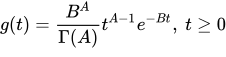
The gamma density function is:
The gamma function Γ(*) is:
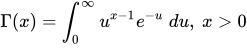
If A is an integer then Γ(A)=(A-1)! where x! is factorial x.
When A = 1 this gives an exponential distribution. If you vary A then the shape of the distribution will change. Changing B does not affect the shape of the distribution, just its scale on the x axis.
Illustration
Suppose you want 100 random values from a gamma distribution with a shaping parameter A = 2 and a scaling parameter B = 3, for example to simulate waiting times that have a mean of 6 and a right skewed spread.
To generate them in StatsDirect select Gamma from the Random Numbers section of the Generating section of the Data menu. Enter 1 as the number of columns to fill and 100 as the number of rows, 2 for A and 3 for B, and enter 1234 as the seed in place of the one suggested. A column headed "Gamma (seed 1234, A = 2, B = 3)" is written to the workbook; the same seed gives the same column again.
For this distribution, where Γ(2) = 1! = 1 so that g(t) = t e-t/3/9:
Mean = 6 (AB)
Variance = 18 (AB2)
Standard deviation = 4.242641
Density at t = 4: 0.117154
P(t <= 4) = 0.38494
Median = 5.035041
95th centile = 14.231594
A sample of 100 values generated in R (see the R code below) had:
Sample mean = 6.599323
Sample sd = 4.681867
The column that StatsDirect writes for seed 1234 has mean 6.021564 and standard deviation 4.184212.
The sample mean is 0.6 above the mean of the distribution, well within the sampling variation to expect from 100 values (the standard error of the mean is 4.24/10 = 0.42). The values that StatsDirect writes differ from R's for any seed, because each program seeds its generator in its own way, but a column of 100 gamma deviates from either should have a mean near 6, a standard deviation near 4.24 and a right skewed histogram with its peak near (A-1)B = 3.
The special cases above can be checked from the cumulative probabilities:
A = 1: P(t <= 4) = 0.736403 (the exponential distribution with mean 3 gives 0.736403)
A = 0.5, B = 1: P(t <= 1.5) = 0.916735 (the chi-square distribution with 1 degree of freedom gives 0.916735 for a squared standard normal deviate of at most 3)
These figures were calculated in R, whose dgamma, pgamma, qgamma and rgamma functions define shape and scale as StatsDirect defines A and B. StatsDirect itself only generates the random numbers, so the probabilities and quantiles do not appear in a StatsDirect report.
See random number fill.

 R code
This R code reproduces the illustration above, apart from the column that StatsDirect writes for seed 1234, whose values R's generator does not repeat. It needs no packages and was checked with R 4.6.1. Paste it into R, or save it as a script and run it.
# Gamma distribution: the StatsDirect help illustration (100 random values with a
# shaping parameter A = 2 and a scaling parameter B = 3, from Data_Generating_Random
# Numbers_Gamma) in R
A <- 2                                    # shaping parameter: R's shape argument
B <- 3                                    # scaling parameter: R's scale argument, the
                                          # reciprocal of its rate argument
six <- function(x) formatC(x, digits = 6, format = "f", drop0trailing = TRUE)

# The distribution: its mean is AB and its variance A times B squared; dgamma, pgamma
# and qgamma give the density, the cumulative probability and the quantiles
cat("Mean =", six(A * B), "  Variance =", six(A * B^2),
    "  Standard deviation =", six(sqrt(A) * B), "\n")
cat("Density at t = 4:", six(dgamma(4, shape = A, scale = B)), "\n")
cat("P(t <= 4) =", six(pgamma(4, shape = A, scale = B)), "\n")
cat("Median =", six(qgamma(0.5, shape = A, scale = B)), "\n")
cat("95th centile =", six(qgamma(0.95, shape = A, scale = B)), "\n")

# 100 random values: R and StatsDirect both use the Mersenne Twister generator but each
# seeds it in its own way, so the values differ from the column StatsDirect fills for
# any seed, while each seed repeats its own series in both programs. The set.seed call
# makes this run repeatable.
set.seed(2024)
x <- rgamma(100, shape = A, scale = B)
print(summary(x))
cat("Sample mean =", six(mean(x)), "  Sample sd =", six(sd(x)), "\n")

# Two special cases the topic mentions: A = 1 is the exponential distribution with
# mean B, and with B = 1, A = 0.5 is half a squared standard normal deviate (half
# a chi-square deviate with 1 degree of freedom), so the cumulative probabilities
# agree
cat("A = 1: P(t <= 4) =", six(pgamma(4, shape = 1, scale = B)),
    " exponential:", six(pexp(4, rate = 1 / B)), "\n")
cat("A = 0.5, B = 1: P(t <= 1.5) =", six(pgamma(1.5, shape = 0.5)),
    " chi-square:", six(pchisq(2 * 1.5, df = 1)), "\n")