Wei-Lachin Test
Menu location: Analysis_Survival_Wei-Lachin.
This function gives a two sample distribution free method for the comparison of two multivariate distributions of survival (time-to-event) data that may be censored (incomplete, e.g. alive at end of study or lost to follow up). Multivariate methods such as this should be used only with expert statistical guidance.
Wei and Lachin generalise the Log-rank and Gehan generalised Wilcoxon tests (using a random censorship model) for multivariate survival data with two main groups. (Makuch and Escobar, 1991; Wei and Lachin, 1984).
Data preparation
StatsDirect asks you for a group identifier, this could be a column of 1 and 2 representing the two groups. You then select k pairs of survival time (time-to-event) and censorship columns for k repeat times. Censored data are coded as 0 and uncensored data are coded as 1.
Repeat times may represent separate factors or the observation of the same factor repeated on k occasions. For example, time to develop symptoms could be analysed for k different symptoms in a group of patients treated with drug x and compared with a group of patients not treated with drug x.
Missing data can be coded either by entering a missing data symbol * as the time, or by setting censored equal to 0 and time less than the minimum uncensored time in your data set.
For further details please refer to Makuch and Escobar (1991) and Wei and Lachin (1984).
Technical Validation
Wei and Lachin's multivariate tests are calculated for the case of two multivariate distributions, and the intermediate univariate statistics are given. The algorithm used for the method is that given by Makuch and Escobar (1991).
The general univariate statistic for comparing the time to event (of component type k out of m multivariate components) of the two groups is calculated as:
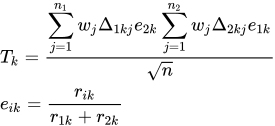
- where n1 is the number of subjects in group 1; n2 is the number of subjects in group 2; n is the total number of subjects; rik is the number at risk in group i at the jth event time in the kth component; Δ is equal to 0 if an observation is censored or 1 otherwise; eik is the expected proportion of events in group i for the kth component; and wj is equal to 1 for the log-rank method or (r1k+r2k)/n for the Gehan-Breslow generalised Wilcoxon method.
The univariate statistic for the kth component of the multivariate survival data is calculated as:
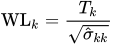
- where σ hatkk is the kth diagonal element of the estimated variance-covariance matrix that is calculated as described by Makuch and Escobar (1991).
An omnibus test that the two multivariate distributions are equal is calculated as:

- where T' is the transpose of the vector of univariate test statistics and Σ-1 is the generalised inverse of the estimated variance-covariance matrix.
A stochastic ordering test statistic is calculated as:
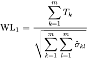
Both one sided and two sided P values are given with the stochastic ordering (linear combination) statistic; some authors prefer one sided inference (Davis, 1994). If you make a one sided inference then you are considering only ascending or only descending ordering, and you are assuming that observing an order in the opposite direction to that expected would be unimportant to your conclusions.
The univariate and stochastic ordering statistics are asymptotically normally distributed; the omnibus statistic is asymptotically chi-square distributed on m degrees of freedom.
Example
From Makuch and Escobar (1991).
Test workbook (Survival worksheet: Treatment Gp, time m1, censor m1, time m2, censor m2, time m3, censor m3, time m4, censor m4).
The following data represent the times in days it took in vitro cultures of lymphocytes to reach a level of p24 antigen expression. The cultures were taken from patients infected with HIV-1 who had advanced AIDS or AIDS related complex. The idea was that patients whose cultures took a short time to express p24 antigen had a greater load of HIV-1. The two groups represented patients on two different treatments. The culture was run for 30 days and specimens which remained negative or which became contaminated were called censored (=0). The tests were run over four 30 day periods.
| Treatment Gp | time m1 | censor m1 | time m2 | censor m2 | time m3 | censor m3 | time m4 | censor m4 |
| 1 | 8 | 1 | 0 | 0 | 25 | 0 | 21 | 1 |
| 1 | 6 | 1 | 4 | 1 | 5 | 1 | 5 | 1 |
| 1 | 6 | 1 | 5 | 1 | 28 | 0 | 18 | 1 |
| 1 | 14 | 0 | 35 | 0 | 23 | 1 | 19 | 0 |
| 1 | 7 | 1 | 0 | 0 | 13 | 1 | 0 | 0 |
| 1 | 5 | 1 | 4 | 1 | 27 | 1 | 8 | 1 |
| 1 | 5 | 1 | 21 | 0 | 6 | 1 | 14 | 1 |
| 1 | 6 | 1 | 10 | 1 | 14 | 1 | 18 | 1 |
| 1 | 7 | 1 | 4 | 1 | 15 | 1 | 8 | 1 |
| 1 | 6 | 1 | 5 | 1 | 5 | 1 | 5 | 1 |
| 1 | 4 | 1 | 5 | 1 | 6 | 1 | 3 | 1 |
| 1 | 5 | 1 | 4 | 1 | 7 | 1 | 5 | 1 |
| 1 | 21 | 0 | 5 | 1 | 0 | 0 | 6 | 1 |
| 1 | 13 | 1 | 27 | 0 | 21 | 0 | 8 | 1 |
| 1 | 4 | 1 | 27 | 0 | 7 | 1 | 6 | 1 |
| 1 | 6 | 1 | 3 | 1 | 7 | 1 | 8 | 1 |
| 1 | 6 | 1 | 0 | 0 | 5 | 1 | 5 | 1 |
| 1 | 6 | 1 | 0 | 0 | 4 | 1 | 6 | 1 |
| 1 | 7 | 1 | 9 | 1 | 6 | 1 | 7 | 1 |
| 1 | 8 | 1 | 15 | 1 | 8 | 1 | 0 | 0 |
| 1 | 18 | 0 | 27 | 0 | 18 | 0 | 9 | 1 |
| 1 | 16 | 1 | 14 | 1 | 14 | 1 | 6 | 1 |
| 1 | 15 | 1 | 9 | 1 | 12 | 1 | 12 | 1 |
| 2 | 4 | 1 | 5 | 1 | 4 | 1 | 3 | 1 |
| 2 | 8 | 1 | 22 | 1 | 25 | 0 | 0 | 0 |
| 2 | 6 | 1 | 6 | 1 | 8 | 1 | 5 | 1 |
| 2 | 7 | 1 | 10 | 1 | 10 | 1 | 18 | 1 |
| 2 | 5 | 1 | 14 | 1 | 17 | 0 | 6 | 1 |
| 2 | 3 | 1 | 5 | 1 | 8 | 1 | 6 | 1 |
| 2 | 6 | 1 | 11 | 1 | 6 | 1 | 13 | 1 |
| 2 | 6 | 1 | 0 | 0 | 15 | 1 | 7 | 1 |
| 2 | 6 | 1 | 12 | 1 | 19 | 1 | 8 | 1 |
| 2 | 6 | 1 | 25 | 0 | 0 | 0 | 22 | 0 |
| 2 | 4 | 1 | 7 | 1 | 5 | 1 | 7 | 1 |
| 2 | 5 | 1 | 7 | 1 | 4 | 1 | 6 | 1 |
| 2 | 3 | 1 | 9 | 1 | 7 | 1 | 6 | 1 |
| 2 | 9 | 1 | 17 | 1 | 0 | 0 | 21 | 0 |
| 2 | 6 | 1 | 4 | 1 | 8 | 1 | 14 | 1 |
| 2 | 5 | 1 | 5 | 1 | 7 | 1 | 16 | 0 |
| 2 | 12 | 1 | 18 | 0 | 14 | 1 | 0 | 0 |
| 2 | 9 | 1 | 11 | 1 | 15 | 1 | 18 | 0 |
| 2 | 6 | 1 | 5 | 1 | 9 | 1 | 0 | 0 |
| 2 | 18 | 0 | 8 | 1 | 10 | 1 | 13 | 1 |
| 2 | 4 | 1 | 4 | 1 | 5 | 1 | 10 | 1 |
| 2 | 3 | 1 | 10 | 1 | 0 | 0 | 21 | 0 |
| 2 | 8 | 1 | 7 | 1 | 10 | 1 | 12 | 1 |
| 2 | 3 | 1 | 6 | 1 | 7 | 1 | 9 | 1 |
To analyse these data in StatsDirect you must first prepare them in 9 workbook columns as shown above. Alternatively, open the test workbook using the file open function of the file menu. Then select Wei-Lachin from the Survival Analysis section of the analysis menu. Select the column marked "Treatment Gp" when asked for the group identifier. Next, enter the number of repeat times as four. Select "time m1" and "censor m1" for time and censorship for repeat time one. Repeat this selection process for the other three repeat times.
For this example:
Wei-Lachin analysis
Univariate Generalised Wilcoxon (Gehan)
total cases = 47 (by group = 23 and 24)
Repeat time 1
observed failures by group = 20 and 23
Wei-Lachin t = -0.527597
Wei-Lachin variance = 0.077575
chi-square = 3.588261 P = 0.0582
Repeat time 2
observed failures by group = 14 and 21
Wei-Lachin t = 0.077588
Wei-Lachin variance = 0.056161
chi-square = 0.107189 P = 0.7434
Repeat time 3
observed failures by group = 18 and 19
Wei-Lachin t = -0.11483
Wei-Lachin variance = 0.060918
chi-square = 0.216452 P = 0.6418
Repeat time 4
observed failures by group = 20 and 16
Wei-Lachin t = 0.335179
Wei-Lachin variance = 0.056281
chi-square = 1.996143 P = 0.1577
Multivariate Generalised Wilcoxon (Gehan)
Covariance matrix:
| 0.077575 | |||
| 0.026009 | 0.056161 | ||
| 0.035568 | 0.020484 | 0.060918 | |
| 0.023525 | 0.016862 | 0.026842 | 0.056281 |
Inverse of covariance matrix:
| 19.204259 | |||
| -5.078483 | 22.22316 | ||
| -8.40436 | -3.176864 | 25.857118 | |
| -2.497583 | -3.020025 | -7.867237 | 23.468861 |
repeat times = 4
chi-square omnibus statistic = 9.242916 P = 0.0553
stochastic ordering z = -0.30981 one sided P = 0.3784, two sided P = 0.7567
Univariate Log-Rank
total cases = 47 (by group = 23 and 24)
Repeat time 1
observed failures by group = 20 and 23
Wei-Lachin t = -0.716191
Wei-Lachin variance = 0.153385
chi-square = 3.344058 P = 0.0674
Repeat time 2
observed failures by group = 14 and 21
Wei-Lachin t = -0.277786
Wei-Lachin variance = 0.144359
chi-square = 0.534536 P = 0.4647
Repeat time 3
observed failures by group = 18 and 19
Wei-Lachin t = -0.372015
Wei-Lachin variance = 0.150764
chi-square = 0.917956 P = 0.338
Repeat time 4
observed failures by group = 20 and 16
Wei-Lachin t = 0.619506
Wei-Lachin variance = 0.143437
chi-square = 2.675657 P = 0.1019
Multivariate Log-Rank
Covariance matrix:
| 0.153385 | |||
| 0.049439 | 0.144359 | ||
| 0.052895 | 0.050305 | 0.150764 | |
| 0.039073 | 0.047118 | 0.052531 | 0.143437 |
Inverse of covariance matrix:
| 7.973385 | |||
| -1.779359 | 8.69056 | ||
| -1.892007 | -1.661697 | 8.575636 | |
| -0.894576 | -1.761494 | -2.079402 | 8.555558 |
repeat times = 4
chi-square omnibus statistic = 9.52966 P = 0.0491
stochastic ordering z = -0.688754 one sided P = 0.2455, two sided P = 0.491
Here the multivariate log-rank test has revealed a statistically significant difference between the treatment groups which was not revealed by any of the individual univariate tests. For more detailed discussion of each result parameter see Wei and Lachin (1984).

 R code
This R code reproduces the example above. It uses the survival package, which comes with R, and was checked with R 4.6.1. Paste it into R, or save it as a script and run it.
# Wei-Lachin test: the StatsDirect help example (Makuch and Escobar 1991, days for
# lymphocyte cultures from 47 HIV patients in two treatment groups to express p24
# antigen, over four periods) in R. The data are the test workbook's Survival worksheet
# columns Treatment Gp, time m1, censor m1, ... time m4, censor m4.
p24 <- data.frame(
  Treatment.Gp = c(1, 1, 1, 1, 1, 1, 1, 1, 1, 1, 1, 1, 1, 1, 1, 1, 1, 1, 1, 1,
    1, 1, 1, 2, 2, 2, 2, 2, 2, 2, 2, 2, 2, 2, 2, 2, 2, 2, 2, 2, 2, 2, 2, 2, 2,
    2, 2),
  time.m1 = c(8, 6, 6, 14, 7, 5, 5, 6, 7, 6, 4, 5, 21, 13, 4, 6, 6, 6, 7, 8, 18,
    16, 15, 4, 8, 6, 7, 5, 3, 6, 6, 6, 6, 4, 5, 3, 9, 6, 5, 12, 9, 6, 18, 4, 3,
    8, 3),
  censor.m1 = c(1, 1, 1, 0, 1, 1, 1, 1, 1, 1, 1, 1, 0, 1, 1, 1, 1, 1, 1, 1, 0,
    1, 1, 1, 1, 1, 1, 1, 1, 1, 1, 1, 1, 1, 1, 1, 1, 1, 1, 1, 1, 1, 0, 1, 1, 1, 1),
  time.m2 = c(0, 4, 5, 35, 0, 4, 21, 10, 4, 5, 5, 4, 5, 27, 27, 3, 0, 0, 9, 15,
    27, 14, 9, 5, 22, 6, 10, 14, 5, 11, 0, 12, 25, 7, 7, 9, 17, 4, 5, 18, 11, 5,
    8, 4, 10, 7, 6),
  censor.m2 = c(0, 1, 1, 0, 0, 1, 0, 1, 1, 1, 1, 1, 1, 0, 0, 1, 0, 0, 1, 1, 0,
    1, 1, 1, 1, 1, 1, 1, 1, 1, 0, 1, 0, 1, 1, 1, 1, 1, 1, 0, 1, 1, 1, 1, 1, 1, 1),
  time.m3 = c(25, 5, 28, 23, 13, 27, 6, 14, 15, 5, 6, 7, 0, 21, 7, 7, 5, 4, 6,
    8, 18, 14, 12, 4, 25, 8, 10, 17, 8, 6, 15, 19, 0, 5, 4, 7, 0, 8, 7, 14, 15,
    9, 10, 5, 0, 10, 7),
  censor.m3 = c(0, 1, 0, 1, 1, 1, 1, 1, 1, 1, 1, 1, 0, 0, 1, 1, 1, 1, 1, 1, 0,
    1, 1, 1, 0, 1, 1, 0, 1, 1, 1, 1, 0, 1, 1, 1, 0, 1, 1, 1, 1, 1, 1, 1, 0, 1, 1),
  time.m4 = c(21, 5, 18, 19, 0, 8, 14, 18, 8, 5, 3, 5, 6, 8, 6, 8, 5, 6, 7, 0,
    9, 6, 12, 3, 0, 5, 18, 6, 6, 13, 7, 8, 22, 7, 6, 6, 21, 14, 16, 0, 18, 0,
    13, 10, 21, 12, 9),
  censor.m4 = c(1, 1, 1, 0, 0, 1, 1, 1, 1, 1, 1, 1, 1, 1, 1, 1, 1, 1, 1, 0, 1,
    1, 1, 1, 0, 1, 1, 1, 1, 1, 1, 1, 0, 1, 1, 1, 0, 1, 0, 0, 0, 0, 1, 1, 0, 1, 1))
group <- p24$Treatment.Gp
times <- as.matrix(p24[, paste0("time.m", 1:4)])
censor <- as.matrix(p24[, paste0("censor.m", 1:4)])   # 1 = event, 0 = censored

# One repeat time on its own is an ordinary two-group survival comparison, which the
# survival package (it comes with R) tests with survdiff(): rho = 0 is the log-rank
# test and rho = 1 the Peto-Peto version of the Wilcoxon test. Their chi-squares differ
# from the Wei-Lachin univariate ones below, which weight by the proportion at risk
# (Gehan) and use Wei and Lachin's variance estimate rather than the hypergeometric one
if (!requireNamespace("survival", quietly = TRUE)) install.packages("survival", repos = "https://cloud.r-project.org")
library(survival)
print(survdiff(Surv(times[, 1], censor[, 1]) ~ group))

# Neither base R nor the survival package has the Wei-Lachin test, so it is computed by
# the formulae above, following Makuch and Escobar (1991). For each repeat time and
# each event, e is the expected share of the event for each group (its number at risk
# over the total at risk), weighted by w: 1 for the log-rank method, or the proportion
# of subjects at risk for Gehan's generalised Wilcoxon method. Each subject then has a
# score for each repeat time (its weighted expected share for the other group if it had
# an event, less the running sum psi of the expected shares of the events in its own
# group at or before its own time, each divided by the number of its group then at
# risk), and the covariance matrix of the statistics is the mean cross product of these
# scores
six <- function(x) formatC(x, digits = 6, format = "f", drop0trailing = TRUE)
pv <- function(p) {
  if (p < 0.0001) "P < 0.0001" else
    paste("P =", formatC(p, digits = 4, format = "f", drop0trailing = TRUE))
}
wei_lachin <- function(times, censor, group, gehan) {
  g <- match(group, unique(group))   # the groups numbered in order of first appearance
  n <- nrow(times)
  m <- ncol(times)
  t_k <- numeric(m)
  failures <- matrix(0, 2, m)
  scores <- matrix(0, n, m)
  for (k in 1:m) {
    x <- times[, k]
    s <- censor[, k]
    y1 <- sapply(x, function(t) sum(g == 1 & x >= t))   # at risk in each group at
    y2 <- sapply(x, function(t) sum(g == 2 & x >= t))   # each subject's own time
    w <- if (gehan) (y1 + y2) / n else 1
    e1 <- ifelse(s == 1, w * y1 / (y1 + y2), 0)
    e2 <- ifelse(s == 1, w * y2 / (y1 + y2), 0)
    mu <- ifelse(g == 1, e2, e1)      # the expected share for the other group
    t_k[k] <- (sum(mu[g == 1]) - sum(mu[g == 2])) / sqrt(n)
    failures[, k] <- tabulate(g[s == 1], 2)
    y_own <- ifelse(g == 1, y1, y2)
    psi <- sapply(1:n, function(j) {
      earlier <- g == g[j] & s == 1 & x <= x[j]
      sum(mu[earlier] / y_own[earlier])
    })
    scores[, k] <- mu - psi
  }
  sigma <- crossprod(scores) / n
  list(n = n, by_group = tabulate(g, 2), failures = failures, t = t_k, sigma = sigma)
}

# The report gives the Gehan (generalised Wilcoxon) results first, then the log-rank
# ones. The univariate chi-square is (t / standard error)^2; the omnibus statistic is
# t' inverse(sigma) t on m degrees of freedom, and the stochastic ordering z is the sum
# of the t over the square root of the sum of the whole covariance matrix. solve()
# needs the covariance matrix to be of full rank, as it is here (StatsDirect uses a
# generalised inverse, which is the same when the matrix is of full rank)
lower <- function(a) {
  for (i in seq_len(nrow(a))) cat(six(a[i, 1:i]), "\n")
}
for (gehan in c(TRUE, FALSE)) {
  method <- if (gehan) "Generalised Wilcoxon (Gehan)" else "Log-Rank"
  wl <- wei_lachin(times, censor, group, gehan)
  m <- length(wl$t)
  cat("\nUnivariate", method, "\n")
  cat("total cases = ", wl$n, " (by group = ", wl$by_group[1], " and ", wl$by_group[2],
      ")\n", sep = "")
  for (k in 1:m) {
    chi <- wl$t[k]^2 / wl$sigma[k, k]
    cat("Repeat time", k, "\n")
    cat("observed failures by group =", wl$failures[1, k], "and", wl$failures[2, k],
        "\n")
    cat("Wei-Lachin t =", six(wl$t[k]), "\n")
    cat("Wei-Lachin variance =", six(wl$sigma[k, k]), "\n")
    cat("chi-square =", six(chi), " ", pv(pchisq(chi, 1, lower.tail = FALSE)), "\n")
  }
  cat("\nMultivariate", method, "\n")
  cat("Covariance matrix:\n")
  lower(wl$sigma)
  cat("Inverse of covariance matrix:\n")
  lower(solve(wl$sigma))
  omnibus <- drop(t(wl$t) %*% solve(wl$sigma) %*% wl$t)
  cat("repeat times =", m, "\n")
  cat("chi-square omnibus statistic =", six(omnibus), " ",
      pv(pchisq(omnibus, m, lower.tail = FALSE)), "\n")
  z <- sum(wl$t) / sqrt(sum(wl$sigma))
  p1 <- pnorm(-abs(z))
  cat("stochastic ordering z = ", six(z), "  one sided ", pv(p1), ",  two sided ",
      pv(2 * p1), "\n", sep = "")
}