Follow-up Life Table
Menu location: Analysis_Survival_Follow-Up Life Table.
This function provides a follow-up life table that displays the survival experience of a cohort.
The table is constructed by the following definitions:
- Interval
- For a Berkson and Gage survival table this is the survival times in intervals.
- For an abridged life table this is ages in groups.
- Deaths
- Number of individuals who die in the interval. [dx]
- Withdrawn
- Number of individuals withdrawn or lost to follow up in the interval. [wx]
- At Risk
- Number of individuals alive at the start of the interval. [nx]
- Adj. at risk
- Adjusted number at risk (half of withdrawals of current interval subtracted). [n'x]
- P(death)
- Probability that an individual who survived the last interval will die in the current interval. [qx]
- P(survival)
- Probability that an individual who survived the last interval will survive the current interval. [px]
- % Survivors (lx)
- Probability of an individual surviving to the start of the current interval (beyond all earlier intervals).
- Proportion of survivors at the start of the current interval.
- Life table survival rate.
- SD of lx%
- Standard deviation of lx% from Greenwood's formula. The confidence interval is calculated on the log(-log lx) scale, so it is not lx% plus or minus 1.96 times this.
- *% CI for lx%
- *% confidence interval for lx%.
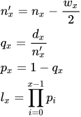
- where lx is the product of all px before x.
Technical validation
The Berkson and Gage method is used to construct the basic table (Berkson and Gage, 1950; Armitage and Berry, 1994; Altman, 1991; Lawless, 1982; Kalbfleisch and Prentice, 1980; Le, 1997). The confidence interval for lx is not a simple application of the estimated variance for lx, instead it uses a maximum likelihood solution from an asymptotic distribution by the transformation of lx suggested by Kalbfleisch and Prentice (1980). This treatment of lx avoids impossible values (i.e. >1 or <0).
Example
From Armitage and Berry (1994, p. 473).
Test workbook (Survival worksheet: Year, Died, Withdrawn).
The following data represent the survival of 374 patients who had one type of surgery for a particular malignancy.
| Years since operation (start of interval) | Died in this interval | Lost to follow-up |
| 0 | 90 | 0 |
| 1 | 76 | 0 |
| 2 | 51 | 0 |
| 3 | 25 | 12 |
| 4 | 20 | 5 |
| 5 | 7 | 9 |
| 6 | 4 | 9 |
| 7 | 1 | 3 |
| 8 | 3 | 5 |
| 9 | 2 | 5 |
| 10 | 21 | 26 |
To analyse these data in StatsDirect you must first prepare them in three workbook columns appropriately labelled. Alternatively, open the test workbook using the file open function of the file menu. Then select Follow-up Life Table from the survival analysis section of the analysis menu. Select the column marked "Year" when asked for the times, select "Died" when asked for deaths and "Withdrawn" when asked for withdrawals. Select 374 (total deaths and withdrawals) as the number alive at the start.
For this example:
Follow-up life table
| Interval | Deaths | Withdrawn | At risk | Adj. at risk | P(death) |
| 0 to 1 | 90 | 0 | 374 | 374 | 0.240642 |
| 1 to 2 | 76 | 0 | 284 | 284 | 0.267606 |
| 2 to 3 | 51 | 0 | 208 | 208 | 0.245192 |
| 3 to 4 | 25 | 12 | 157 | 151 | 0.165563 |
| 4 to 5 | 20 | 5 | 120 | 117.5 | 0.170213 |
| 5 to 6 | 7 | 9 | 95 | 90.5 | 0.077348 |
| 6 to 7 | 4 | 9 | 79 | 74.5 | 0.053691 |
| 7 to 8 | 1 | 3 | 66 | 64.5 | 0.015504 |
| 8 to 9 | 3 | 5 | 62 | 59.5 | 0.05042 |
| 9 to 10 | 2 | 5 | 54 | 51.5 | 0.038835 |
| 10 up | 21 | 26 | 47 | * | * |
| Interval | P(survival) | Survivors (lx%) | SD of lx% | 95% CI for lx% |
| 0 to 1 | 0.759358 | 100 | * | * to * |
| 1 to 2 | 0.732394 | 75.935829 | 2.210411 | 71.271289 to 79.951252 |
| 2 to 3 | 0.754808 | 55.614973 | 2.569084 | 50.428392 to 60.482341 |
| 3 to 4 | 0.834437 | 41.97861 | 2.551951 | 36.945565 to 46.922332 |
| 4 to 5 | 0.829787 | 35.028509 | 2.479272 | 30.200182 to 39.889161 |
| 5 to 6 | 0.922652 | 29.066209 | 2.388987 | 24.47156 to 33.805 |
| 6 to 7 | 0.946309 | 26.817994 | 2.350474 | 22.322081 to 31.504059 |
| 7 to 8 | 0.984496 | 25.378102 | 2.331928 | 20.935141 to 30.043836 |
| 8 to 9 | 0.94958 | 24.984643 | 2.328731 | 20.552912 to 29.648834 |
| 9 to 10 | 0.961165 | 23.724913 | 2.322116 | 19.323326 to 28.39237 |
| 10 up | * | 22.803557 | 2.321531 | 18.417247 to 27.483099 |
We conclude with 95% confidence that the true population survival rate 5 years after the surgical operation studied is between 24.5% and 33.8% for people diagnosed as having this cancer.

 R code
This R code reproduces the example above. It needs no packages and was checked with R 4.6.1. Paste it into R, or save it as a script and run it.
# Follow-up (actuarial) life table: the StatsDirect help example (Armitage and Berry
# 1994, the survival of 374 patients after surgery for a malignancy; the test workbook's
# Survival worksheet columns Year, Died and Withdrawn) in R
year <- 0:10
died <- c(90, 76, 51, 25, 20, 7, 4, 1, 3, 2, 21)
withdrawn <- c(0, 0, 0, 12, 5, 9, 9, 3, 5, 5, 26)
alive_at_start <- 374         # StatsDirect's default: the deaths plus the withdrawals

# Base R and the survival package have no actuarial life table (survfit() gives the
# Kaplan-Meier estimate, which treats each death time individually), so the Berkson and
# Gage table is computed from its formulae: the number at risk in an interval is reduced
# by half the withdrawals of that interval, and the probability of surviving beyond an
# interval is the product of the interval survival probabilities up to it. The last
# interval is open ended, so its probability of death is not estimated and the table
# stops at the survival to its start (StatsDirect prints * for these cells)
six <- function(x) formatC(x, digits = 6, format = "f", drop0trailing = TRUE)
star <- function(x) ifelse(is.na(x), "*", six(x))
k <- length(year)
closed <- 1:(k - 1)
at_risk <- alive_at_start - c(0, cumsum(died + withdrawn)[-k])
adj_at_risk <- at_risk - withdrawn / 2
q <- died[closed] / adj_at_risk[closed]
p <- 1 - q
lx <- cumprod(p)
interval <- c(paste(year[closed], "to", year[-1]), paste(year[k], "up"))
cat("Follow-up life table\n")
print(data.frame(Interval = interval, Deaths = died, Withdrawn = withdrawn,
                 "At risk" = at_risk, "Adj. at risk" = star(c(adj_at_risk[closed], NA)),
                 "P(death)" = star(c(q, NA)), check.names = FALSE), row.names = FALSE)

# Greenwood's formula gives the variance of lx, and the report's column "SD of lx%" is
# 100 times its square root. The confidence interval is on the scale of log(-log(lx)),
# the transformation of Kalbfleisch and Prentice (1980), so that its limits stay between
# 0 and 100%. lx and its interval in each row are the survival to the start of the row.
# These lines hold while some die and some survive in every closed interval (0 < q < 1),
# as here; StatsDirect prints * for the cells that are not estimable otherwise
var_lx <- lx^2 * cumsum(q / (adj_at_risk[closed] * p))
s <- sqrt(var_lx) / (-lx * log(lx))
z <- qnorm(0.975)
lower <- 100 * lx^exp(z * s)
upper <- 100 * lx^exp(-z * s)
ci <- c("* to *", paste(six(lower), "to", six(upper)))
print(data.frame(Interval = interval, "P(survival)" = star(c(p, NA)),
                 "Survivors (lx%)" = six(100 * c(1, lx)),
                 "SD of lx%" = star(c(NA, 100 * sqrt(var_lx))),
                 "95% CI for lx%" = ci, check.names = FALSE), row.names = FALSE)