Sample Size for Survival Analysis
Menu location: Analysis_Sample Size_Survival Times.
This function gives you the minimum number of subjects that you require to detect a true hazard ratio (hr) for experimental subjects relative to controls with power POWER and two sided type I error probability ALPHA (Dupont, 1990; Schoenfeld and Richter, 1982).
The method used here is suitable for calculating sample sizes for studies that will be analysed by the log-rank test.
Information required
- POWER: probability of detecting a real effect.
- ALPHA: probability of detecting a false effect (two sided: double this if you need one sided).
- A: accrual time during which subjects are recruited to the study.
- F: additional follow-up time after the end of recruitment.
- *: input either (C and r) or (C and E), where r=C/E.
- C: median survival time for control group.
- E: median survival time for experimental group.
- r: hazard ratio for experimental subjects relative to controls, which is C/E with exponential survival.
- M: number of controls per experimental subject.
Practical issues
- Usual values for POWER are 80%, 85% and 90%; try several in order to explore/scope.
- 5% is the usual choice for ALPHA.
- C is usually estimated from previous studies.
- If possible, choose a range of hazard ratios that you want to have the statistical power to detect.
Technical validation
The estimated number of experimental subjects n (with mn controls) is calculated as:
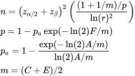
- where α = alpha, β = 1 - power, m is the number of controls per experimental subject and zp is the standard normal deviate for probability p. n is rounded up to the next whole number. (1+1/m)/p is equivalent to 2/p in the first equation if the experimental and control group sizes are equal (m = 1).
Example
Suppose you plan a trial of a new treatment against the usual one, with death as the endpoint. From earlier studies the median survival on the usual treatment is about 12 months, and you want to be able to detect an improvement to a median of 18 months on the new treatment (a hazard ratio of 0.67), with 80% power at the 5% two sided level. You expect to recruit for 24 months and to follow the subjects for another 12 months after the last one is recruited, allocating one control per experimental subject. The figures are invented for this illustration.
To run this in StatsDirect select Survival Times from the Sample Size section of the Analysis menu. Enter 12 as the median survival time in the control group, choose to enter two median survival times and enter 18 for the experimental group, then 24 as the accrual time, 12 as the additional follow-up time, 1 as the number of controls per experimental subject, 80% as the power and 5% as alpha.
For this example:
Sample size for survival analysis
median survival time for controls = 12
median survival time for experimental subjects = 18
hazard ratio (experimental vs. control) = 0.666667
accrual time for recruitment = 24
additional follow-up time after recruitment = 12
alpha = 0.05
power = 0.8
Estimated minimum sample size = 147 experimental subjects and 147 controls
The trial would need 147 subjects in each group, 294 in all. The number depends on how many deaths the study will observe, not only on how many subjects it recruits: if instead the trial recruited for 36 months and closed as soon as recruitment ended, so that the last subjects recruited were hardly followed at all, 187 in each group would be needed for the same power.

 R code
This R code reproduces the example above. It needs no packages and was checked with R 4.6.1. Paste it into R, or save it as a script and run it.
# Sample size for survival analysis: the StatsDirect help example (an invented trial
# of a new treatment against the usual one: median survival 12 months on the usual
# treatment, 18 months hoped for on the new one, two years of recruitment and one
# more year of follow-up) in R
ct <- 12                                  # median survival time in the control group
et <- 18                                  # median survival time, experimental group
at <- 24                                  # accrual time, when subjects are recruited
fut <- 12                                 # further follow-up time after recruitment
m <- 1                                    # controls per experimental subject
power <- 0.8
alpha <- 0.05                             # two sided

# Neither base R nor the survival package has a function for this sample size, so the
# topic's formula (Schoenfeld and Richter 1982) is written out here. Survival is taken
# to be exponential in both groups, so the hazard ratio is the inverse ratio of the
# median survival times. A subject recruited at a uniformly distributed time during
# accrual is followed for less than the whole study, and the power of the log-rank test
# depends on how many deaths are seen before the study ends.
six <- function(x) formatC(x, digits = 6, format = "f", drop0trailing = TRUE)
size_survival <- function(ct, et, at, fut, m, power, alpha) {
  hr <- ct / et                           # experimental hazard relative to controls
  tbar <- (ct + et) / 2                   # the average of the two median survival times
  k <- log(2) * at / tbar
  pa <- (1 - exp(-k)) / k                 # probability of surviving the accrual period,
                                          # averaged over the recruitment times
  p <- 1 - pa * exp(-log(2) * fut / tbar) # probability of dying before the study ends
  n <- (qnorm(1 - alpha / 2) + qnorm(power))^2 * ((1 + 1 / m) / p) / log(hr)^2
  n <- floor(n) + 1                       # next whole number (one above an exact n)
  cat("median survival time for controls =", six(ct), "\n")
  cat("median survival time for experimental subjects =", six(et), "\n")
  cat("hazard ratio (experimental vs. control) =", six(hr), "\n")
  cat("accrual time for recruitment =", six(at), "\n")
  cat("additional follow-up time after recruitment =", six(fut), "\n")
  cat("alpha =", six(alpha), "\n")
  cat("power =", six(power), "\n")
  cat("Estimated minimum sample size =", n, "experimental subjects and",
      ceiling(n * m), "controls\n\n")
}
size_survival(ct, et, at, fut, m, power, alpha)

# The same trial recruiting for three years and closing as soon as recruitment ends:
# fewer of the deaths are seen by then, so more subjects are needed for the same power
size_survival(ct, et, at = 36, fut = 0, m, power, alpha)