Sample Size for Paired Cohort Studies
Menu location: Analysis_Sample Size_Paired Cohort.
This function gives you the minimum number of subject pairs that you require to detect a true relative risk RR with power POWER and two sided type I error probability ALPHA (Dupont, 1990; Breslow and Day, 1980).
Information required
- POWER: probability of detecting a real effect.
- ALPHA: probability of detecting a false effect (two sided: double this if you need one sided).
- r: correlation coefficient for failure between paired subjects.
- *: input either (P0 and RR) or (P0 and P1), where RR=P1/P0.
- P0: event rate in the control group.
- P1: event rate in experimental group.
- RR: risk of failure of experimental subjects relative to controls.
Practical issues
- Usual values for POWER are 80%, 85% and 90%; try several in order to explore/scope.
- 5% is the usual choice for ALPHA.
- r can be estimated from previous studies - note that r is the phi (correlation) coefficient that is given for a two by two table if you enter it into the StatsDirect r by c chi-square function. When r is not known from previous studies, some authors state that it is better to use a small arbitrary value for r, say 0.2, than it is to assume independence (a value of 0) (Dupont, 1988).
- P0 can be estimated as the population event rate. Note, however, that due to matching, the control sample is not a random sample from the population therefore population event rate can be a poor estimate of P0 (especially if confounders are strongly associated with the event).
- If possible, choose a range of relative risks that you want to have the statistical power to detect.
Technical validation
The estimated sample size n is calculated as:
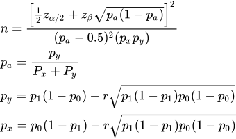
- where α = alpha, β = 1 - power and zp is the standard normal deviate for probability p. n is rounded up to the closest integer.
Example
Consider a planned cohort study in which each worker exposed to a solvent is matched, on age and sex, with an unexposed worker from the same industry, and both are followed for the same period for a skin condition. Earlier studies suggest that about 10% of unexposed workers develop the condition. The investigators want a 90% chance of detecting a doubling of the risk with exposure (a relative risk of 2) with a two sided test at the 5% level. The correlation for failure between the paired subjects is not known, so it is taken as 0.2 as suggested above. These figures are invented for illustration.
To calculate the sample size in StatsDirect select Paired Cohort from the Sample Size section of the Analysis menu. Enter 0.1 as the event rate in the control group, choose Relative Risk and enter 2, enter 0.2 as the correlation coefficient, then 90% for power and 5% for alpha.
For this example:
Sample size for paired cohort study
Event rate in control group = 0.1
Event rate in experimental group = 0.2
Correlation for failure between experimental and control subjects = 0.2
Alpha = 0.05
Power = 0.9
Estimated minimum sample size = 203 pairs
So 203 matched pairs, 406 workers in all, are needed. Entering the event rate in the experimental group as 0.2 instead of the relative risk gives the same result. Try other values of power, alpha and correlation to see how sensitive the size is to them.

 R code
This R code reproduces the example above. It needs no packages and was checked with R 4.6.1. Paste it into R, or save it as a script and run it.
# Sample size for a paired cohort study: the StatsDirect help example (an invented study
# of exposed workers each matched with an unexposed worker, 10% of controls with the
# event, a relative risk of 2 to be detected) in R
p0 <- 0.1                                 # event rate in the control group
rr <- 2                                   # relative risk to be detected
p1 <- rr * p0                             # event rate in the experimental group, 0.2
r <- 0.2                                  # correlation for failure within a pair
power <- 0.9
alpha <- 0.05                             # two sided

# Base R's power.prop.test() is for two independent groups and takes no account of the
# pairing, so the topic's formula (Dupont 1990, from Breslow and Day 1980) is used: the
# probabilities of the two kinds of discordant pair, the proportion of discordant pairs
# in which the experimental subject is the one who fails, then the number of pairs,
# rounded up. It needs p1 to differ from p0 and both discordant probabilities to be
# positive (r not too large), which is why StatsDirect refuses some inputs.
z_alpha <- qnorm(1 - alpha / 2)           # two sided: 1.959964 for alpha 0.05
z_beta <- qnorm(power)                    # 1.281552 for 90% power
s <- r * sqrt(p1 * (1 - p1) * p0 * (1 - p0))
py <- p1 * (1 - p0) - s                   # experimental subject fails, control does not
px <- p0 * (1 - p1) - s                   # control fails, experimental subject does not
stopifnot(p1 != p0, px > 0, py > 0)
pa <- py / (px + py)
n <- (z_alpha / 2 + z_beta * sqrt(pa * (1 - pa)))^2 / ((pa - 0.5)^2 * (px + py))
cat("Event rate in control group =", p0, "\n")
cat("Event rate in experimental group =", p1, "\n")
cat("Correlation for failure between experimental and control subjects =", r, "\n")
cat("Alpha =", alpha, "\n")
cat("Power =", power, "\n")
cat("Estimated minimum sample size =", ceiling(n), "pairs\n")