Sample Size for Matched Case-control Studies
Menu location: Analysis_Sample Size_Matched Case-Control.
This function gives you the minimum sample size necessary to detect a true odds ratio OR with power POWER and a two sided type I error probability ALPHA. If you are using more than one control per case then this function also provides the reduction in sample size relative to a paired study that you can obtain using your number of controls per case (Dupont, 1988).
Information required
- POWER: probability of detecting a real effect.
- ALPHA: probability of detecting a false effect (two sided: double this if you need one sided).
- r: correlation coefficient (ϕ) for exposure between matched cases and controls.
- P0: probability of exposure in the control group.
- m: number of control subjects matched to each case subject.
- OR: odds ratio (ψ).
Practical issues
- Usual values for POWER are 80%, 85% and 90%; try several in order to explore/scope.
- 5% is the usual choice for ALPHA.
- r can be estimated from previous studies - note that r is the phi (correlation) coefficient that is given for a two by two table if you enter it into the StatsDirect r by c chi-square function. When r is not known from previous studies, some authors state that it is better to use a small arbitrary value for r, say 0.2, than it is to assume independence (a value of 0) (Dupont, 1988).
- P0 can be estimated as the population prevalence of exposure. Note, however, that due to matching, the control sample is not a random sample from the population therefore population prevalence of exposure can be a poor estimate of P0 (especially if confounders are strongly associated with exposure, Dupont, 1988).
- If possible, choose a range of odds ratios that you want to have the statistical power to detect.
Technical validation
The estimated sample size n is calculated as (Dupont, 1990):
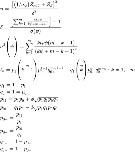
- where α = alpha, β = 1 - power, ψ = odds ratio, ϕ is the correlation coefficient for exposure between matched cases and controls, and Zp is the standard normal deviate for probability p. n is rounded up to the closest integer.
Example
Suppose you plan a case-control study of whether an exposure in childhood raises the odds of a disease in adult life, with three controls matched to each case for age and sex. From earlier surveys you expect 30% of the controls to have been exposed, you want to be able to detect an odds ratio of 2, and you allow for a correlation of 0.2 for exposure between a case and its matched controls rather than assuming independence. You want 80% power with a two sided alpha of 5%. The figures are invented for this illustration.
To run this in StatsDirect select Matched Case-Control from the Sample Size section of the Analysis menu. Enter 0.2 as the correlation coefficient, 0.3 as the probability of exposure in the control group, 2 as the odds ratio and 3 as the number of controls per case, then 80% as the power and 5% as alpha.
For this example:
Sample size for matched case-control study
case-control correlation = 0.2
probability of exposure in controls = 0.3
odds ratio = 2
controls per case subject = 3
alpha = 0.05
power = 0.8
Estimated minimum sample size (cases required) = 108
Reduction in sample size, relative to paired design,
when using 3 controls per case = 0.6
Running the function again with 1 as the number of controls per case, the other entries unchanged, gives:
Sample size for matched case-control study
case-control correlation = 0.2
probability of exposure in controls = 0.3
odds ratio = 2
controls per case subject = 1
alpha = 0.05
power = 0.8
Estimated minimum sample size (cases required) = 180
With three controls per case, 108 cases (and 324 controls) would give 80% power to detect an odds ratio of 2. With one control per case 180 cases would be needed, so the extra controls reduce the number of cases to 60% of that of the paired design. The saving diminishes as further controls are added to each case.

 R code
This R code reproduces the example above. It needs no packages and was checked with R 4.6.1. Paste it into R, or save it as a script and run it.
# Sample size for a matched case-control study: the StatsDirect help example (an
# invented study with three controls matched to each case, exposure in 30% of the
# controls, an odds ratio of 2 to detect and a correlation of 0.2 for exposure
# between a case and its controls) in R
phi <- 0.2                                # correlation of exposure within a matched set
p0 <- 0.3                                 # probability of exposure in the controls
psi <- 2                                  # odds ratio to be detected
m <- 3                                    # controls matched to each case
power <- 0.8
alpha <- 0.05                             # two sided

# Base R has no function for this design, so the formulae in the topic (Dupont 1988)
# are used. First the probability of exposure in the cases, p1: the odds ratio is
# that of the discordant case-control pairs, p10 / p01, where p01 is as the topic
# gives it and p10 = p1 q0 - phi sqrt(p1 q1 p0 q0), so p1 is the value that makes
# this ratio equal to psi (found numerically here; the program solves the same
# equation)
exposure_odds <- function(p1) {
  s <- phi * sqrt(p1 * (1 - p1) * p0 * (1 - p0))
  (p1 * (1 - p0) - s) - psi * ((1 - p1) * p0 - s)
}
p1 <- uniroot(exposure_odds, c(1e-8, 1 - 1e-8), tol = 1e-12)$root
q0 <- 1 - p0
q1 <- 1 - p1
s <- phi * sqrt(p1 * q1 * p0 * q0)
# every cell of the case-control exposure table must be a probability
stopifnot(p1 * p0 + s >= 0, p1 * q0 - s >= 0, q1 * p0 - s >= 0, q1 * q0 + s >= 0)
p0_plus <- (p1 * p0 + s) / p1             # exposure in a control of an exposed case
p0_minus <- (q1 * p0 - s) / q1            # exposure in a control of an unexposed case

# The cases needed with m controls per case: t_k is the probability that k of the m + 1
# members of a matched set are exposed (sets with none or all exposed carry no
# information); the score statistic has mean E and variance V per matched set, at the
# odds ratio to detect and, for the null hypothesis, at an odds ratio of 1
cases_needed <- function(m) {
  k <- 1:m
  t_k <- p1 * choose(m, k - 1) * p0_plus^(k - 1) * (1 - p0_plus)^(m - k + 1) +
    q1 * choose(m, k) * p0_minus^k * (1 - p0_minus)^(m - k)
  E <- function(psi) sum(k * t_k * psi / (k * psi + m - k + 1))
  V <- function(psi) sum(k * t_k * psi * (m - k + 1) / (k * psi + m - k + 1)^2)
  z_alpha <- qnorm(1 - alpha / 2)
  z_beta <- qnorm(power)
  (z_alpha * sqrt(V(1)) + z_beta * sqrt(V(psi)))^2 / (E(psi) - E(1))^2
}
six <- function(x) formatC(x, digits = 6, format = "f", drop0trailing = TRUE)
n_m <- ceiling(cases_needed(m))           # rounded up to a whole number of cases
n_1 <- ceiling(cases_needed(1))           # the paired design, one control per case
cat("case-control correlation =", phi, "\n")
cat("probability of exposure in controls =", p0, "\n")
cat("odds ratio =", psi, "\n")
cat("controls per case subject =", m, "\n")
cat("alpha =", alpha, "\n")
cat("power =", power, "\n")
cat("Estimated minimum sample size (cases required) =", n_m, "\n")
cat("Reduction in sample size, relative to paired design,\n")
cat("when using", m, "controls per case =", six(n_m / n_1), "\n")

# The paired design itself, for comparison
cat("controls per case subject = 1\n")
cat("Estimated minimum sample size (cases required) =", n_1, "\n")