Sample Size for Pearson's Correlation
Menu location: Analysis_Sample Size_Correlation.
This function gives you the minimum number of pairs of subjects needed to detect a true difference in Pearson's correlation coefficient between the null (usually 0) and alternative hypothesis levels with power POWER and two sided type I error probability ALPHA (Stuart and Ord, 1994; Draper and Smith, 1998).
Information required
- POWER: probability of detecting a true effect.
- ALPHA: probability of detecting a false effect (two sided: double this if you need one sided).
- R0: correlation coefficient under the null hypothesis (often 0; StatsDirect takes R0 and R1 between 0 and 1, so if both are negative enter their absolute values).
- R1: correlation coefficient under the alternative hypothesis.
Practical issues
- Usual values for POWER are 80%, 85% and 90%; try several in order to explore/scope.
- 5% is the usual choice for ALPHA.
- Two sided in this context means R0 not equal to R1, one sided would be R1 either greater than or less than R0 which is rarely appropriate because you can seldom say that a difference in the unexpected direction would be of no interest at all.
- Statistical correlation can be misleading, remember to think beyond the numerical association between two variables, and not to infer causality too easily.
Technical validation
The sample size estimation uses Fisher's classic z-transformation to normalise the distribution of Pearson's correlation coefficient:
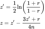
This gives rise to the usual test for an observed correlation coefficient (r1) to be tested for its difference from a pre-defined reference value (r0, often 0), and from this the power and sample size (n) can be determined:

StatsDirect makes an initial estimate of n as:
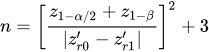
StatsDirect then finds the value of n that satisfies the following power (1-β) equation:
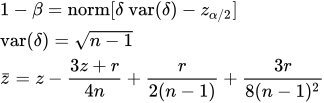
-where norm is the area under the standard normal distribution curve.
The initial estimate is rounded up to a whole number and then moved to the smallest number of pairs at which the power equation gives at least the required power; this is the sample size given by StatsDirect.
Example
Suppose that you are planning a study of the association between two measurements, and that a correlation of 0.4 or more would matter in practice. This is an invented example: you want an 80% chance of detecting a true correlation of 0.4 at the two sided 5% level of significance, against the null hypothesis of no correlation (R0 = 0).
To calculate this in StatsDirect select Correlation from the Sample Size section of the Analysis menu. Enter 0 as the correlation coefficient under the null hypothesis and 0.4 as the correlation coefficient under the alternative hypothesis, then 80% as the power and 5% as alpha.
For this example:
Sample size for Pearson correlation
Alpha = 0.05
Power = 0.8
Correlation coefficient under null hypothesis = 0
Correlation coefficient under alternative hypothesis = 0.4
Estimated minimum sample size = 47
The initial estimate from the formula above is 46.73 pairs, which is rounded up to 47. With 47 pairs the power equation gives 80.2%, and with 46 pairs 79.3%, so 47 is the smallest number of pairs that meets the target: the study should include at least 47 pairs of measurements.

 R code
This R code reproduces the example above. It needs no packages and was checked with R 4.6.1. Paste it into R, or save it as a script and run it.
# Sample size for Pearson's correlation: the StatsDirect help example (an invented
# study that should detect a correlation of 0.4 or more, r1 = 0.4 against the null
# value r0 = 0, with 80% power at the two sided 5% level) in R
r0 <- 0
r1 <- 0.4
power <- 0.8
alpha <- 0.05
stopifnot(r0 != r1, abs(r0) < 1, abs(r1) < 1)  # Fisher's z needs |r| < 1, r0 != r1

# Base R has no function for this sample size, so the topic's method is used here.
# Fisher's z transformation, atanh(r) = 0.5 * log((1 + r) / (1 - r)), makes a sample
# correlation from n pairs approximately normal with mean atanh(rho) and variance
# 1 / (n - 3), which gives the two sided power of a test between the two hypotheses.
dif <- abs(atanh(r1) - atanh(r0))
z_alpha <- qnorm(1 - alpha / 2)
z_power <- qnorm(power)
size_power <- function(n) {
  z <- dif * sqrt(n - 3)
  pnorm(z - z_alpha) + pnorm(-z - z_alpha)
}

# The initial estimate ((z_alpha + z_power) / dif)^2 + 3 is rounded up, then moved to
# the smallest whole number of pairs (at least 4) at which the power reaches the target
n0 <- ((z_alpha + z_power) / dif)^2 + 3
n <- max(ceiling(n0), 4)
while (n > 4 && size_power(n - 1) >= power) n <- n - 1
while (size_power(n) < power) n <- n + 1
cat("Alpha =", alpha, "\n")
cat("Power =", power, "\n")
cat("Correlation coefficient under null hypothesis =", r0, "\n")
cat("Correlation coefficient under alternative hypothesis =", r1, "\n")
cat("Estimated minimum sample size =", n, "\n")

# The working: the initial estimate and the power either side of the answer
pct <- function(x) paste0(formatC(100 * x, digits = 1, format = "f"), "%")
cat("Initial estimate of n =", formatC(n0, digits = 2, format = "f"), "\n")
cat("Power with", n - 1, "pairs =", paste0(pct(size_power(n - 1)), ","), "with", n,
    "pairs =", pct(size_power(n)), "\n")