Partial Correlation
Partial correlation is a method used to describe the relationship between two variables whilst taking away the effects of another variable, or several other variables, on this relationship.
Partial correlation is best thought of in terms of multiple regression; StatsDirect shows the partial correlation coefficient r with its main results from multiple linear regression.
A different way to calculate partial correlation coefficients, which does not require a full multiple regression, is show below for the sake of further explanation of the principles:
Consider a correlation matrix for variables A, B and C (note that the multiple linear regression function in StatsDirect will output correlation matrices for you as one of its options):
| A | B | C | |
| A: | * | ||
| B: | r(AB) | * | |
| C: | r(AC) | r(BC) | * |
The partial correlation of A and B adjusted for C is:
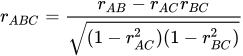
The same can be done using Spearman's rank correlation co-efficient.
The hypothesis test for the partial correlation co-efficient is performed in the same way as for the usual correlation co-efficient but it is based upon n-3 degrees of freedom.
Please note that this sort of relationship between three or more variables is more usefully investigated using the multiple regression itself (Altman, 1991).
The general form of partial correlation from a multiple regression is as follows:
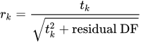
- where tk is the Student t statistic for the kth term in the linear model.
Example
For the multiple linear regression example (Armitage and Berry, 1994: recovery time YY after a hypotensive drug against the log dose X1 and the mean blood pressure X2 of 53 patients) the multiple regression report gives the partial correlation of each predictor with the outcome, adjusted for the other predictor, beside its coefficient:
X1: r = 0.438695, t = 3.45194, P = 0.0011
X2: r = -0.317915, t = -2.371006, P = 0.0216
The first formula above gives the same values from the three pairwise correlations of YY, X1 and X2, and the second gives them from the t statistics with the 50 residual degrees of freedom.

 R code
This R code reproduces the illustration above. It needs no packages and was checked with R 4.6.1. Paste it into R, or save it as a script and run it.
# Partial correlation: the multiple linear regression topic's example (Armitage and
# Berry 1994, recovery time YY after a hypotensive drug against the log dose X1 and
# the mean blood pressure X2 of 53 patients) in R
yy <- c(7, 10, 18, 4, 10, 13, 21, 12, 9, 65, 20, 31, 23, 22, 13, 9, 50, 12, 11, 8, 26,
        16, 23, 7, 11, 8, 14, 39, 28, 12, 60, 10, 60, 22, 21, 14, 4, 27, 26, 28, 15, 8,
        46, 24, 12, 25, 45, 72, 25, 28, 10, 25, 44)
x1 <- c(2.26, 1.81, 1.78, 1.54, 2.06, 1.74, 2.56, 2.29, 1.80, 2.32, 2.04, 1.88, 1.18,
        2.08, 1.70, 1.74, 1.90, 1.79, 2.11, 1.72, 1.74, 1.60, 2.15, 2.26, 1.65, 1.63,
        2.40, 2.70, 1.90, 2.78, 2.27, 1.74, 2.62, 1.80, 1.81, 1.58, 2.41, 1.65, 2.24,
        1.70, 2.45, 1.72, 2.37, 2.23, 1.92, 1.99, 1.99, 2.35, 1.80, 2.36, 1.59, 2.10,
        1.80)
x2 <- c(66, 52, 72, 67, 69, 71, 88, 68, 59, 73, 68, 58, 61, 68, 69, 55, 67, 67, 68, 59,
        68, 63, 65, 72, 58, 69, 70, 73, 56, 83, 67, 84, 68, 64, 60, 62, 76, 60, 60, 59,
        84, 66, 68, 65, 69, 72, 63, 56, 70, 69, 60, 51, 61)

# From the correlation matrix, as the topic's first formula: the partial
# correlation of YY and X1 adjusted for X2
r <- cor(cbind(yy, x1, x2))
partial <- function(ab, ac, bc) (ab - ac * bc) / sqrt((1 - ac^2) * (1 - bc^2))
six <- function(x) formatC(x, digits = 6, format = "f", drop0trailing = TRUE)
cat("r(YY, X1 | X2) =", six(partial(r["yy", "x1"], r["yy", "x2"], r["x1", "x2"])), "\n")
cat("r(YY, X2 | X1) =", six(partial(r["yy", "x2"], r["yy", "x1"], r["x1", "x2"])), "\n")

# From the multiple regression, as the topic's second formula: t over root(t squared
# plus the residual degrees of freedom), the r the report prints beside each term
fit <- lm(yy ~ x1 + x2)
t <- summary(fit)$coefficients[, "t value"]
df <- fit$df.residual
cat("From the regression: X1 r =", six(t["x1"] / sqrt(t["x1"]^2 + df)), " X2 r =",
    six(t["x2"] / sqrt(t["x2"]^2 + df)), "\n")

# The test of a partial correlation has n - 3 degrees of freedom here (one
# adjusting variable); its P is the t test of the term in the regression
pv <- function(p) {
  if (p < 0.0001) "P < 0.0001" else
    paste("P =", formatC(p, digits = 4, format = "f", drop0trailing = TRUE))
}
for (term in c("x1", "x2")) {
  cat(toupper(term), ": t =", six(t[term]), "on", df, "DF, two sided",
      pv(2 * pt(-abs(t[term]), df)), "\n")
}