Compare Two Crude Rates
Menu location: Analysis_Rates_Compare Two Crude Rates.
Person-time data from prospective studies of two groups with different exposures may be expressed as a difference between incidence rates or as a ratio of incidence rates.
This function constructs confidence intervals for incidence rate differences and ratios where there are two exposures (i.e. exposed or not exposed, defined according to certain risk factors) (Sahai and Khurshid, 1996).
Data input
| EXPOSURE: | |||
| Exposed | Not Exposed | ||
| OUTCOME: | Cases: | a | b |
| Person-time: | PT1 | PT2 | |
The use of person-time as opposed to just "time" enables you to handle situations where there are drop-outs in a study or where you have not been able to follow an entire cohort at risk to watch for the development of the outcome under investigation. Thus, the follow up period does not have to be uniform for all participants. Person-time for a group is the sum of the times of follow up for each participant in that group.
Technical validation
The confidence interval for the rate difference is constructed from the standard error of the difference, where each rate has the variance of a Poisson count divided by the square of its person-time. The chi-square statistic tests the equality of the two rates, given the total number of events. The confidence interval for the rate ratio is exact, using the Poisson distribution (Sahai and Khurshid, 1996):
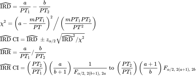
- where IRD hat and IRR hat are point estimates of incidence rate difference and ratio respectively, m is the total number of events observed, PT is the total person-time observed, Z is a quantile of the standard normal distribution and F is a quantile of the F distribution (denominator degrees of freedom are quoted last).
The optional conditional maximum likelihood analysis for the rate ratio employs the polynomial multiplication method described by Martin and Austin (1996); this also provides mid-P estimates.
Example
From Stampfer et al. (1985).
| Postmenopausal hormone use: | ||
| Yes | No | |
| CHD cases: | 30 | 60 |
| Person-years: | 54308.7 | 51477.5 |
For this example:
| EXPOSURE | |||
| Exposed | Non-exposed | Total | |
| Cases: | 30 | 60 | 90 |
| Person-time: | 54308.7 | 51477.5 | 105786.2 |
Exposed incidence rate = 0.000552
Non-exposed incidence rate = 0.001166
Rate difference = -0.000613
Approximate 95% confidence interval = -0.000968 to -0.000258
Chi-square = 11.678635 P = 0.0006
Rate ratio = 0.473934
Exact 95% confidence interval = 0.295128 to 0.746416
Conditional maximum likelihood estimate of rate ratio = 0.473934
Exact Fisher 95% confidence interval = 0.295128 to 0.746416
Exact Fisher one sided P = 0.0004, two sided P = 0.0007
Exact mid-P 95% confidence interval = 0.302362 to 0.730939
Exact mid-P one sided P = 0.0003, two sided P = 0.0006
Here we may conclude with 95% confidence that the true population value for the difference between the two incidence rates lies somewhere between -0.001 and -0.0003. We may also conclude with 95% confidence that the incidence rate for those who used postmenopausal hormones in the circumstances of the study was between 0.30 and 0.75 of that for those who did not take postmenopausal hormones.

 R code
This R code reproduces the example above. It needs no packages and was checked with R 4.6.1. Paste it into R, or save it as a script and run it.
# Compare two crude rates: the StatsDirect help example (Stampfer et al. 1985, cases of
# coronary heart disease and person-years of follow up among users and non-users of
# postmenopausal hormones) in R
a <- 30          # cases among the exposed (hormone users)
b <- 60          # cases among the non-exposed
pt1 <- 54308.7   # person-years of follow up of the exposed
pt2 <- 51477.5   # person-years of follow up of the non-exposed

# R's standard comparison of two rates. It conditions on the total number of cases:
# if the two rates were equal, the exposed cases a would be binomial with probability
# pt1 / (pt1 + pt2), so the comparison is the exact binomial test of a in a + b. Its
# rate ratio is the report's rate ratio and its conditional maximum likelihood
# estimate. Its interval is the Clopper-Pearson binomial interval turned into a rate
# ratio, which is the report's exact (Fisher) interval. Its P value is the report's
# two sided exact Fisher P (the binomial test of a in a + b, two sided).
print(poisson.test(c(a, b), c(pt1, pt2)))

# The rates and their difference. Each rate has the variance of a Poisson count
# divided by the square of its person-time, so the standard error of the difference
# is the square root of a / pt1^2 + b / pt2^2, and the limits are the difference
# plus or minus z times that standard error. The chi-square statistic compares a
# with its expected value given the total number of cases
six <- function(x) formatC(x, digits = 6, format = "f", drop0trailing = TRUE)
pv <- function(p) {
  if (p < 0.0001) "P < 0.0001" else
    paste("P =", formatC(p, digits = 4, format = "f", drop0trailing = TRUE))
}
m <- a + b
pt <- pt1 + pt2
ir1 <- a / pt1
ir2 <- b / pt2
ird <- ir1 - ir2
cat("Exposed incidence rate =", six(ir1), "\n")
cat("Non-exposed incidence rate =", six(ir2), "\n")
se <- sqrt(a / pt1^2 + b / pt2^2)
z <- qnorm(0.975)
cat("Rate difference =", six(ird), "\n")
cat("approximate 95% confidence interval =", six(ird - z * se), "to",
    six(ird + z * se), "\n")
chisq <- (a - m * pt1 / pt)^2 / (m * pt1 * pt2 / pt^2)
cat("chi-square =", six(chisq), " ", pv(pchisq(chisq, 1, lower.tail = FALSE)), "\n")

# The rate ratio and its exact interval from quantiles of the F distribution, as the
# formula above gives it. The lower limit is 0 when a is 0 and the upper limit is
# infinite when b is 0. The limits agree with those of poisson.test to 6 places.
irr <- ir1 / ir2
lower <- if (a == 0) 0 else pt2 / pt1 * (a / (b + 1)) / qf(0.975, 2 * (b + 1), 2 * a)
upper <- if (b == 0) Inf else pt2 / pt1 * ((a + 1) / b) * qf(0.975, 2 * (a + 1), 2 * b)
cat("Rate ratio =", six(irr), "\n")
cat("exact 95% confidence interval =", six(lower), "to", six(upper), "\n")

# The conditional analysis. Given the total m, a is binomial with probability
# p = pt1 * ratio / (pt1 * ratio + pt2), and a rate ratio is recovered from a
# probability p as p * pt2 / ((1 - p) * pt1). The one sided Fisher P is the smaller
# tail of that distribution at a ratio of 1; the two sided P adds up the probabilities
# of the values of a that are no more probable than the one observed.
ratio <- function(p) p * pt2 / ((1 - p) * pt1)
cat("Conditional maximum likelihood estimate of rate ratio =", six(irr), "\n")
cat("Exact Fisher 95% confidence interval =", six(lower), "to", six(upper), "\n")
prob <- dbinom(0:m, m, pt1 / pt)
up <- sum(prob[(a + 1):(m + 1)])
down <- sum(prob[1:(a + 1)])
two <- sum(prob[prob <= prob[a + 1] * (1 + 1e-7)])
cat("Exact Fisher one sided ", pv(min(up, down)), ", two sided ", pv(two), "\n",
    sep = "")

# The mid-P versions count half of the probability of a itself: each limit is the
# probability at which the tail beyond a plus half the probability of a is 2.5%,
# found by root finding, and the two sided mid-P is twice the one sided value
mid_tail <- function(p, top) {
  half <- 0.5 * dbinom(a, m, p)
  if (top) pbinom(a - 1, m, p) + half else pbinom(a, m, p, lower.tail = FALSE) + half
}
lower_mid <- if (a == 0) 0 else
  ratio(uniroot(function(p) mid_tail(p, FALSE) - 0.025, c(1e-12, 1 - 1e-12),
                tol = 1e-12)$root)
upper_mid <- if (b == 0) Inf else
  ratio(uniroot(function(p) mid_tail(p, TRUE) - 0.025, c(1e-12, 1 - 1e-12),
                tol = 1e-12)$root)
cat("Exact mid-P 95% confidence interval =", six(lower_mid), "to", six(upper_mid),
    "\n")
mid <- min(up, down) - 0.5 * prob[a + 1]
cat("Exact mid-P one sided ", pv(mid), ", two sided ", pv(min(2 * mid, 1)), "\n",
    sep = "")