Z (Normal Distribution) Tests
Menu locations:
Analysis_Parametric_Single Sample z
Analysis_Parametric_Unpaired z
For large (50 or more observations) normally distributed samples, normal distribution tests are equivalent to Student t tests.
Normal data
You may either compare the means of two independent random samples or compare the mean of one sample with a known population mean. Note that for large degrees of freedom, Student's t distribution is approximately normal (Altman, 1991; Armitage and Berry, 1994).
See the examples for t tests and consider these in the context of larger samples.
You will gain a little more sensitivity by using a normal distribution test instead of its equivalent Student t test but you must have good reason to believe that your data have been drawn from a normal distribution. Student t tests are less sensitive than normal distribution tests to small deviations from normality; use t tests if you have any doubt. If your data are clearly non-normal then you should consider using a nonparametric alternative such as the Wilcoxon signed ranks test or the Mann-Whitney U test.
The single sample test statistic is calculated as:

- where x bar is the sample mean, s² is the sample variance, n is the sample size, µ is the specified population mean and z is a quantile from the standard normal distribution.
The unpaired test statistic is calculated as:
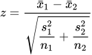
- where x-bar 1 and x-bar 2 are the sample means, s1² and s2² are the sample variances, n1 and n2 are the sample sizes and z is a quantile from the standard normal distribution.
Log-normal data
For samples from a log-normal distribution (logs from a normal distribution) you may wish to construct an interval analogous to the confidence interval for the mean of a sample from a normal distribution. StatsDirect gives you the geometric mean (arithmetic mean of logs) and a reference range as:
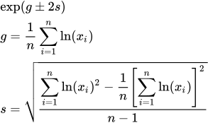
- where g is geometric mean, ln is natural logarithm, n is sample size and z is a quantile from the standard normal distribution (alpha/2 quantile for a 100*(1-alpha)% confidence interval). The geometric mean and its reference range are given only if every value of the sample is above zero.
Example
Test workbook (Parametric worksheet: Michelson).
Consider Michelson's 100 measurements in 1879 of the speed of light in air, in millions of metres per second (Dorsey, 1944), which are also used in the univariate summary example. The accepted value of the speed of light in a vacuum is 299.792458 million metres per second.
To analyse these data in StatsDirect open the test workbook using the file open function of the file menu. Then select Single Sample z from the Parametric section of the Analysis menu. Select the column marked "Michelson" when prompted for data, enter 299.792458 as the population mean and leave the population standard deviation blank.
For this example:
Normal distribution (z) test - single sample
Sample name: Michelson
Sample mean = 299.8524
Population mean = 299.792458
Sample size n = 100
Sample sd = 0.079011
Population sd = not known
95% confidence interval for mean difference = 0.044456 to 0.075428
Standard normal deviate (z) = 7.586582
One sided P < 0.0001
Two sided P < 0.0001
For lognormal data:
Geometric mean = 299.85239 (95% reference range = 299.697571 to 300.007288)
The measurements were on average 0.06 million metres per second above the accepted value in a vacuum, and further above the speed in air, which is about 0.03% lower. The confidence interval shows that the variation between measurements does not explain this: the series carried a systematic error, as is well known for these data.
To compare two independent samples, for example the first and the last 50 of these measurements to look for a drift over the series, copy them into two columns (or add a column of group identifiers, 1 for the first 50 and 2 for the rest, and select it as the group identifier). Then select Unpaired z from the Parametric section of the Analysis menu.
Normal distribution (z) test - two independent samples
Sample name: First 50
Mean = 299.8728
Variance = 0.008951
Size = 50
Sample name: Last 50
Mean = 299.832
Variance = 0.002812
Size = 50
Combined standard error = 0.015338
95% confidence interval for difference between means = 0.010737 to 0.070863
Standard normal deviate (z) = 2.659979
One sided P = 0.0039
Two sided P = 0.0078
The later measurements were lower on average, and a difference this large is unlikely to arise by chance. With 50 measurements in each sample the unpaired t test gives almost the same answer (t = 2.66 on 77 degrees of freedom with unequal variances, two sided P = 0.0095).

 R code
This R code reproduces the example above. It needs no packages and was checked with R 4.6.1. Paste it into R, or save it as a script and run it.
# Normal distribution (z) tests: the StatsDirect help example (Michelson's 100
# measurements of the speed of light in air, millions of metres per second) in R
speed <- c(299.85, 299.74, 299.90, 300.07, 299.93, 299.85, 299.95, 299.98, 299.98,
           299.88, 300.00, 299.98, 299.93, 299.65, 299.76, 299.81, 300.00, 300.00,
           299.96, 299.96, 299.96, 299.94, 299.96, 299.94, 299.88, 299.80, 299.85,
           299.88, 299.90, 299.84, 299.83, 299.79, 299.81, 299.88, 299.88, 299.83,
           299.80, 299.79, 299.76, 299.80, 299.88, 299.88, 299.88, 299.86, 299.72,
           299.72, 299.62, 299.86, 299.97, 299.95, 299.88, 299.91, 299.85, 299.87,
           299.84, 299.84, 299.85, 299.84, 299.84, 299.84, 299.89, 299.81, 299.81,
           299.82, 299.80, 299.77, 299.76, 299.74, 299.75, 299.76, 299.91, 299.92,
           299.89, 299.86, 299.88, 299.72, 299.84, 299.85, 299.85, 299.78, 299.89,
           299.84, 299.78, 299.81, 299.76, 299.81, 299.79, 299.81, 299.82, 299.85,
           299.87, 299.87, 299.81, 299.74, 299.81, 299.94, 299.95, 299.80, 299.81,
           299.87)
n <- length(speed)
mu <- 299.792458                          # the accepted value, in a vacuum

# R has no z test among its standard functions (with a sample this large t.test
# gives almost the same answers), so the report's lines are calculated here.
six <- function(x) formatC(x, digits = 6, format = "f", drop0trailing = TRUE)
pv <- function(p) {
  if (p < 0.0001) "P < 0.0001" else paste("P =", formatC(p, digits = 4, format = "f"))
}
z <- qnorm(0.975)
cat("Sample mean =", six(mean(speed)), "  Sample size n =", n,
    "  Sample sd =", six(sd(speed)), "\n")

# Single sample test, with the population sd not known: the sample sd is used
se <- sd(speed) / sqrt(n)
cat("95% confidence interval for mean difference =", six(mean(speed) - mu - z * se),
    "to", six(mean(speed) - mu + z * se), "\n")
dev <- (mean(speed) - mu) / se
cat("Standard normal deviate (z) =", six(dev), "\n")
cat("One sided", pv(pnorm(-abs(dev))), "  Two sided", pv(2 * pnorm(-abs(dev))), "\n")

# For lognormal data: the geometric mean, with the reference range exp(mean of
# the logs plus or minus z times their sd)
lg <- log(speed)
cat("Geometric mean =", six(exp(mean(lg))), " (95% reference range =",
    six(exp(mean(lg) - z * sd(lg))), "to", paste0(six(exp(mean(lg) + z * sd(lg))), ")"),
    "\n")

# Two independent samples: the first and last 50 measurements
first <- speed[1:50]
last <- speed[51:100]
cat("First 50:  Mean =", six(mean(first)), "  Variance =", six(var(first)),
    "  Size =", length(first), "\n")
cat("Last 50:  Mean =", six(mean(last)), "  Variance =", six(var(last)),
    "  Size =", length(last), "\n")
se2 <- sqrt(var(first) / length(first) + var(last) / length(last))
cat("Combined standard error =", six(se2), "\n")
d <- mean(first) - mean(last)
cat("95% confidence interval for difference between means =", six(d - z * se2), "to",
    six(d + z * se2), "\n")
dev2 <- d / se2
cat("Standard normal deviate (z) =", six(dev2), "\n")
cat("One sided", pv(pnorm(-abs(dev2))), "  Two sided", pv(2 * pnorm(-abs(dev2))), "\n")