Reference Range
Menu location: Analysis_Parametric_Reference Range.
This function enables you to construct confidence intervals for a reference range (also known as reference interval or normal range) from a sample of observations drawn at random from a normal distribution. The nonparametric alternative (quantile reference range) is also given.
The reference range and confidence interval for data from a normal distribution is calculated as:
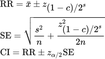
- where x bar is the sample mean, s is the sample standard deviation, n is the sample size, RR is the reference range, SE is the standard error of the reference range limits, CI is the confidence interval for the reference range limits, z is a quantile from the standard normal distribution and c is % range coverage/100 (e.g. 0.95 for a 95% reference range).
For samples with no zero or negative values, the above calculations are repeated on log-transformed data and the results are presented in the original measurement scale.
The reference range and confidence interval for data that are not from a normal distribution should be calculated by the percentile method. For a c*100% reference range, the percentile method examines the (1-c)/2 and 1-(1-c)/2 (i.e. 0.025 and 0.975 for a 95% reference range) sample quantiles and their confidence intervals.
Example
From Altman (1991, p. 421).
Test workbook (Parametric worksheet: IgM).
Consider the serum IgM concentrations measured from blood samples from 298 healthy children aged six months to six years.
To analyse these data in StatsDirect open the test workbook using the file open function of the file menu. Then select the reference range from the parametric methods section of the analysis menu. Select the column marked "IgM" when prompted for data.
For this example:
Reference range/interval
Sample name: IgM
Sample mean = 0.80302
Sample size n = 298
Sample sd = 0.469498
For normal data
95% reference interval = -0.117179 to 1.72322
95% confidence interval for lower range limit = -0.20828 to -0.026079
95% confidence interval for upper range limit = 1.632119 to 1.81432
For log-normal data
95% reference interval = 0.238102 to 2.031412
95% confidence interval for lower range limit = 0.214129 to 0.264758
95% confidence interval for upper range limit = 1.826887 to 2.258836
For any data
Quantile 0.025 = 0.2
Approximate 95% confidence interval (non-conservative) = 0.1 to 0.3
Exact confidence level = 94.120331%
Quantile 0.975 = 2
Approximate 95% confidence interval (non-conservative) = 1.7 to 2.5
Exact confidence level = 94.120331%
These data are not from a normal distribution but are from an approximately log-normal distribution. This explains why the results for log-normal data are closer to the 2.5% and 97.5% percentiles.

 R code
This R code reproduces the example above. It needs no packages and was checked with R 4.6.1. Paste it into R, or save it as a script and run it.
# Reference range: the StatsDirect help example (Altman 1991, serum IgM in 298
# children) in R
# The data are the IgM column of the Parametric worksheet of the StatsDirect test
# workbook.
igm <- c(0.1, 0.1, 0.1, 0.2, 0.2, 0.2, 0.2, 0.2, 0.2, 0.2, 0.3, 0.3, 0.3, 0.3,
  0.3, 0.3, 0.3, 0.3, 0.3, 0.3, 0.3, 0.3, 0.3, 0.3, 0.3, 0.3, 0.3, 0.3, 0.3,
  0.4, 0.4, 0.4, 0.4, 0.4, 0.4, 0.4, 0.4, 0.4, 0.4, 0.4, 0.4, 0.4, 0.4, 0.4,
  0.4, 0.4, 0.4, 0.4, 0.4, 0.4, 0.4, 0.4, 0.4, 0.4, 0.4, 0.4, 0.5, 0.5, 0.5,
  0.5, 0.5, 0.5, 0.5, 0.5, 0.5, 0.5, 0.5, 0.5, 0.5, 0.5, 0.5, 0.5, 0.5, 0.5,
  0.5, 0.5, 0.5, 0.5, 0.5, 0.5, 0.5, 0.5, 0.5, 0.5, 0.5, 0.5, 0.5, 0.5, 0.6,
  0.6, 0.6, 0.6, 0.6, 0.6, 0.6, 0.6, 0.6, 0.6, 0.6, 0.6, 0.6, 0.6, 0.6, 0.6,
  0.6, 0.6, 0.6, 0.6, 0.6, 0.6, 0.6, 0.6, 0.6, 0.6, 0.6, 0.6, 0.6, 0.6, 0.6,
  0.6, 0.6, 0.6, 0.6, 0.7, 0.7, 0.7, 0.7, 0.7, 0.7, 0.7, 0.7, 0.7, 0.7, 0.7,
  0.7, 0.7, 0.7, 0.7, 0.7, 0.7, 0.7, 0.7, 0.7, 0.7, 0.7, 0.7, 0.7, 0.7, 0.7,
  0.7, 0.7, 0.7, 0.7, 0.7, 0.7, 0.7, 0.7, 0.7, 0.7, 0.7, 0.7, 0.8, 0.8, 0.8,
  0.8, 0.8, 0.8, 0.8, 0.8, 0.8, 0.8, 0.8, 0.8, 0.8, 0.8, 0.8, 0.8, 0.8, 0.8,
  0.8, 0.8, 0.8, 0.8, 0.8, 0.8, 0.8, 0.8, 0.8, 0.8, 0.8, 0.8, 0.8, 0.8, 0.8,
  0.8, 0.8, 0.8, 0.8, 0.8, 0.9, 0.9, 0.9, 0.9, 0.9, 0.9, 0.9, 0.9, 0.9, 0.9,
  0.9, 0.9, 0.9, 0.9, 0.9, 0.9, 0.9, 0.9, 0.9, 0.9, 0.9, 0.9, 1, 1, 1, 1, 1, 1,
  1, 1, 1, 1, 1, 1, 1, 1, 1, 1, 1.1, 1.1, 1.1, 1.1, 1.1, 1.1, 1.1, 1.1, 1.1,
  1.1, 1.1, 1.1, 1.1, 1.1, 1.1, 1.1, 1.2, 1.2, 1.2, 1.2, 1.2, 1.2, 1.3, 1.3,
  1.3, 1.3, 1.3, 1.3, 1.3, 1.4, 1.4, 1.4, 1.4, 1.4, 1.4, 1.4, 1.4, 1.4, 1.5,
  1.5, 1.5, 1.5, 1.5, 1.5, 1.6, 1.6, 1.7, 1.7, 1.7, 1.8, 1.8, 1.8, 2, 2, 2, 2.1,
  2.1, 2.2, 2.5, 2.7, 4.5)
n <- length(igm)
z <- qnorm(0.975)                   # for a 95% range and 95% confidence intervals
six <- function(x) formatC(x, digits = 6, format = "f", drop0trailing = TRUE)
cat("Sample mean =", six(mean(igm)), "  Sample size n =", n,
    "  Sample sd =", six(sd(igm)), "\n")

# R has no standard function for a reference range. For data from a normal
# distribution the range is the mean plus or minus z standard deviations, and
# each limit has standard error s * sqrt(1/n + z^2/(2n)) (Altman 1991).
normal_range <- function(x, back = identity) {
  m <- mean(x)
  s <- sd(x)
  limits <- m + c(-1, 1) * z * s
  se <- s * sqrt(1 / n + z^2 / (2 * n))
  cat("95% reference interval =", six(back(limits[1])), "to", six(back(limits[2])),
      "\n")
  cat("95% confidence interval for lower range limit =", six(back(limits[1] - z * se)),
      "to", six(back(limits[1] + z * se)), "\n")
  cat("95% confidence interval for upper range limit =", six(back(limits[2] - z * se)),
      "to", six(back(limits[2] + z * se)), "\n")
}
cat("For normal data\n")
normal_range(igm)
# For log-normal data, the same on the logarithms with the results taken back to
# the original scale (StatsDirect gives this only when no value is 0 or less)
cat("For log-normal data\n")
normal_range(log(igm), exp)

# For any data: the 2.5th and 97.5th percentiles (type 6 in R, as in the quantile
# confidence interval topic) with confidence intervals whose limits are ordered
# values. The number of observations below a population quantile is binomial
# (n, p). With more than 200 observations StatsDirect takes the limits from the
# normal approximation to that distribution, at np plus or minus z sqrt(np(1-p)),
# and then gives the exact probability that they cover the quantile; with fewer
# it searches the binomial distribution itself, as in the quantile topic.
stopifnot(n > 200)
cat("For any data\n")
x <- sort(igm)
for (p in c(0.025, 0.975)) {
  lo <- floor(n * p - z * sqrt(n * p * (1 - p)))   # numbers of values below
  hi <- floor(n * p + z * sqrt(n * p * (1 - p)))
  cat("Quantile", p, "=", quantile(igm, p, type = 6), "\n")
  cat("Approximate 95% confidence interval (non-conservative) =", x[lo + 1], "to",
      x[hi + 1], "\n")
  cat(sprintf("Exact confidence level = %s%%\n",
              six(100 * (pbinom(hi, n, p) - pbinom(lo, n, p)))))
}