Risk Difference Meta-analysis
Menu location: Analysis_Meta-Analysis_Risk Difference.
Case-control studies of dichotomous outcomes (e.g. dead or alive) can be represented by arranging the observed counts into fourfold (2 by 2) tables. Meta-analysis may be used to investigate the combination or interaction of a group of independent studies, for example a series of fourfold tables from similar studies conducted at different centres. This StatsDirect function examines the risk difference within each stratum (a single fourfold table) and across all of the studies/strata.
For a single stratum risk difference is defined as follows:
| EXPOSURE | |||
| Exposed | Non-Exposed | ||
| OUTCOME: | Cases: | a | b |
| Non-cases: | c | d | |
Risk difference = [a/(a+c)] - [b/(b+d)]
For each table the observed risk difference is displayed with a confidence interval. The ’near exact’ method of Miettinen and Nurminen is used to construct the confidence interval (Mee, 1984; Anbar, 1983; Gart and Nam, 1990; Miettinen and Nurminen, 1985; Sahai and Khurshid, 1996). If the ’try exact’ option is not selected then a normal approximation to the confidence interval is given instead.
The Mantel-Haenszel type method of Greenland and Robins (Greenland and Robins, 1985; Sahai and Khurshid, 1996) is used to estimate the pooled risk difference for all strata, assuming a fixed effects model:
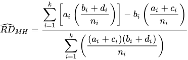
- where ni = ai+bi+ci+di.
A confidence interval for the pooled risk difference is calculated using the Greenland-Robins variance formula (Greenland and Robins, 1985). A chi-square test statistic is given with associated probability of the pooled risk difference being equal to zero. Note that some packages give a z statistic; this is equal to the square root of the chi-square statistic with one degree of freedom, i.e. it is equivalent.
If any cell count in a table is zero then a continuity correction is applied to each cell in that table for the calculation of the weights and variances (the risk difference of the table is calculated from the counts as they are) - if you have selected the 'delay continuity correction' option then the pooled risk difference, its confidence interval and the fixed effects weights are calculated from the counts as they are. The type of continuity correction used is set in the options. A table is left out of the pooling, and marked as excluded, if it has no subjects in one of the groups.
The inconsistency of results across studies is summarised in the I² statistic, which is the percentage of variation across studies that is due to heterogeneity rather than chance – see the heterogeneity section for more information.
Note that the results from StatsDirect may differ slightly from other software or from those quoted in papers; this is due to differences in the variance formulae. StatsDirect employs the most robust practical approaches to variance according to accepted statistical literature.
DATA INPUT:
Observed frequencies should be entered in a workbook as follows:
| Exposed/Experimental | Non-exposed/Non-experimental | ||
| Total number | Number of cases | Total number | Number of cases |
...where total number = cases + non-cases
Example
From Fleiss and Gross (1991).
Test workbook (Meta-analysis worksheet: Exposed total, Exposed cases, Non-exposed total, Non-exposed cases, Study).
The following data combine seven placebo-controlled randomized trials of the effect of aspirin in preventing death after myocardial infarction:
| Aspirin | Placebo | |||
| Trial | patients | deaths | patients | deaths |
| MRC-1 | 615 | 49 | 624 | 67 |
| CDP | 758 | 44 | 771 | 64 |
| MRC-2 | 832 | 102 | 850 | 126 |
| GASP | 317 | 32 | 309 | 38 |
| PARIS | 810 | 85 | 406 | 52 |
| AMIS | 2267 | 246 | 2257 | 219 |
| ISIS-2 | 8587 | 1570 | 8600 | 1720 |
To analyse these data in StatsDirect first prepare them in four workbook columns and label these columns appropriately. Alternatively, open the test workbook using the file open function of the file menu. Then select risk difference from the meta-analysis section of the analysis menu. Select the columns marked "Exposed total", "Exposed cases", "Non-exposed total" and "Non-exposed cases" when prompted for data. Note that "exposed" and "experimental" groups are the same.
For this example:
| Study | Risk difference | 95% CI (Miettinen) | % Weight (fixed, random) | ||
| MRC-1 | -0.027697 | -0.060615 | 0.00482 | 4.445681 | 10.841853 |
| CDP | -0.024962 | -0.051149 | 0.000744 | 5.486129 | 14.756033 |
| MRC-2 | -0.025639 | -0.058485 | 0.007133 | 6.034846 | 10.702518 |
| GASP | -0.022031 | -0.072572 | 0.027778 | 2.245915 | 5.579711 |
| PARIS | -0.023141 | -0.06406 | 0.013999 | 3.881749 | 8.292156 |
| AMIS | 0.011482 | -0.006236 | 0.029241 | 16.233434 | 21.5868 |
| ISIS-2 | -0.017165 | -0.028929 | -0.005404 | 61.672246 | 28.240929 |
Fixed effects (Mantel-Haenszel, Greenland-Robins)
Pooled risk difference = -0.014263 (95% CI = -0.022765 to -0.005762)
Chi² (test risk difference differs from 0) = 10.812247 (df = 1) P = 0.001
Non-combinability of studies
Cochran Q = 10.461119 (df = 6) P = 0.1065
Moment-based estimate of between studies variance = 0.000112
I² (inconsistency) = 42.6% (95% CI = 0% to 77.4%)
Random effects (DerSimonian-Laird)
Pooled risk difference = -0.014947 (95% CI = -0.0276 to -0.002295)
Chi² (test risk difference differs from 0) = 5.361139 (df = 1) P = 0.0206
Bias indicators
Begg-Mazumdar: Kendall's tau = 0.333333 P = 0.3813 (low power)
Egger: bias = -0.817403 (90% CI = -3.132436 to 1.497631) P = 0.5086
Here we can say with 95% confidence, assuming a random effects model, that for those given aspirin the true population risk of dying in the specified interval after a heart attack is at least 0.002 less than the risk for those not given aspirin. Assuming a fixed effects model a stronger inference could be made about a risk difference of 0.006 (the lower absolute confidence limit) but the high inter-study variation makes the fixed effects model less appropriate.

 R code
This R code reproduces the example above. It needs no packages and was checked with R 4.6.1. Paste it into R, or save it as a script and run it.
# Risk difference meta-analysis: the StatsDirect help example (Fleiss and Gross 1991,
# deaths after myocardial infarction in seven placebo-controlled trials of aspirin; the
# test workbook's Meta-analysis worksheet columns A to E) in R
study <- c("MRC-1", "CDP", "MRC-2", "GASP", "PARIS", "AMIS", "ISIS-2")
n1 <- c(615, 758, 832, 317, 810, 2267, 8587)   # aspirin: patients
a <- c(49, 44, 102, 32, 85, 246, 1570)         # aspirin: deaths
n2 <- c(624, 771, 850, 309, 406, 2257, 8600)   # placebo: patients
b <- c(67, 64, 126, 38, 52, 219, 1720)         # placebo: deaths

# Base R has no meta-analysis function, so the statistics are computed from the tables
# as the formulae above give them
six <- function(x) formatC(x, digits = 6, format = "f", drop0trailing = TRUE)
one <- function(x) formatC(x, digits = 1, format = "f", drop0trailing = TRUE)
pv <- function(p) {
  if (p < 0.0001) "P < 0.0001" else
    paste("P =", formatC(p, digits = 4, format = "f", drop0trailing = TRUE))
}
z <- qnorm(0.975)
k <- length(a)
c <- n1 - a
d <- n2 - b
n <- n1 + n2
rd <- a / n1 - b / n2

# The 'near exact' confidence interval of Miettinen and Nurminen (1985) for each study:
# the values of the difference at which the score statistic reaches -1.96 and +1.96,
# with the two proportions estimated under the constraint that they differ by that
# value (the closed form of the constrained estimates, Newcombe 1998 method 10) and
# the variance multiplied by N / (N - 1). These tables have no empty cells; the counts
# of a table with one would have a continuity correction first for the weights and the
# variances further down (but not for its risk difference or for these limits).
mn_limits <- function(a, n1, b, n2) {
  N <- n1 + n2
  score <- function(delta) {
    L3 <- N
    L2 <- (n1 + 2 * n2) * delta - N - a - b
    L1 <- (n2 * delta - N - 2 * b) * delta + a + b
    L0 <- b * delta * (1 - delta)
    q <- L2^3 / (3 * L3)^3 - L1 * L2 / (6 * L3^2) + L0 / (2 * L3)
    p <- sign(q) * sqrt(L2^2 / (3 * L3)^2 - L1 / (3 * L3))
    p2 <- 2 * p * cos((pi + acos(q / p^3)) / 3) - L2 / (3 * L3)
    p1 <- p2 + delta
    v <- (p1 * (1 - p1) / n1 + p2 * (1 - p2) / n2) * N / (N - 1)
    (a / n1 - b / n2 - delta) / sqrt(v)
  }
  est <- a / n1 - b / n2
  c(uniroot(function(x) score(x) - z, c(-1 + 1e-9, est), tol = 1e-12)$root,
    uniroot(function(x) score(x) + z, c(est, 1 - 1e-9), tol = 1e-12)$root)
}
ci <- t(mapply(mn_limits, a, n1, b, n2))

# Mantel-Haenszel weights (fixed effects) and the pooled difference of Greenland and
# Robins (1985), with their variance formula
w_mh <- n1 * n2 / n
rd_mh <- sum(w_mh * rd) / sum(w_mh)
var_mh <- sum((a * c * n2^3 + b * d * n1^3) / (n1 * n2 * n^2)) / sum(w_mh)^2
se_mh <- sqrt(var_mh)

# Cochran's Q about the pooled difference, with inverse variance weights from the
# binomial variances; the DerSimonian-Laird moment estimate of the between studies
# variance and the random effects weights
v_iv <- a * c / n1^3 + b * d / n2^3
w_iv <- 1 / v_iv
q <- sum(w_iv * (rd - rd_mh)^2)
tau2 <- max(0, (q - (k - 1)) / (sum(w_iv) - sum(w_iv^2) / sum(w_iv)))
w_dl <- 1 / (v_iv + tau2)
rd_dl <- sum(w_dl * rd) / sum(w_dl)
se_dl <- 1 / sqrt(sum(w_dl))

# The study table: risk differences, their intervals, their binomial variances and
# the percentage weights
tab <- data.frame(Study = study, `Risk difference` = six(rd), Lower = six(ci[, 1]),
                  Upper = six(ci[, 2]), Variance = six(v_iv),
                  `% fixed` = six(100 * w_mh / sum(w_mh)),
                  `% random` = six(100 * w_dl / sum(w_dl)), check.names = FALSE)
print(tab, row.names = FALSE)

cat("Fixed effects (Mantel-Haenszel, Greenland-Robins)\n")
cat("Pooled risk difference = ", six(rd_mh), " (95% CI = ", six(rd_mh - z * se_mh),
    " to ", six(rd_mh + z * se_mh), ")\n", sep = "")
x2 <- (rd_mh / se_mh)^2
cat("Chi-square (test risk difference differs from 0) =", six(x2), " (df = 1) ",
    pv(pchisq(x2, 1, lower.tail = FALSE)), "\n")

# I-squared = (Q - df) / Q, with the interval StatsDirect gives by default (the 'exact'
# option, Hedges and Pigott 2001): Q is treated as non-central chi-square and its
# distribution function at the observed Q is inverted for the non-centrality parameter
# lambda, the lower limit where that probability is 0.975 (0 when even the central
# distribution gives less) and the upper where it is 0.025; each limit is converted to
# I-squared as lambda / (df + lambda)
cat("Non-combinability of studies\n")
dfree <- k - 1
cat("Cochran Q =", six(q), paste0(" (df = ", dfree, ") "),
    pv(pchisq(q, dfree, lower.tail = FALSE)), "\n")
cat("Moment-based estimate of between studies variance =", six(tau2), "\n")
i2 <- 100 * max(0, (q - dfree) / q)
lambda <- function(p) {
  if (pchisq(q, dfree) < p) 0 else
    uniroot(function(l) pchisq(q, dfree, ncp = l) - p, c(0, 10 * q + 100),
            tol = 1e-10)$root
}
lim <- c(lambda(0.975), lambda(0.025))
cat("I-squared (inconsistency) = ", one(i2), "% (95% CI = ",
    one(100 * lim[1] / (dfree + lim[1])), "% to ",
    one(100 * lim[2] / (dfree + lim[2])), "%)\n", sep = "")

cat("Random effects (DerSimonian-Laird)\n")
cat("Pooled risk difference = ", six(rd_dl), " (95% CI = ", six(rd_dl - z * se_dl),
    " to ", six(rd_dl + z * se_dl), ")\n", sep = "")
x2_dl <- (rd_dl / se_dl)^2
cat("Chi-square (test risk difference differs from 0) =", six(x2_dl), " (df = 1) ",
    pv(pchisq(x2_dl, 1, lower.tail = FALSE)), "\n")

# Bias indicators, both from the binomial variances that the inverse variance weights
# are made from, whatever the method of the intervals of the studies. Begg and
# Mazumdar's test is Kendall's rank correlation between the standardised effects
# (deviations from the inverse variance pooled estimate) and the variances, with the
# exact P that cor.test gives for so few studies when no values tie (fewer than about
# ten gives the test little power). Egger's test regresses the standardised effect
# (estimate / se) on precision (1 / se) and asks whether the intercept is zero, with
# a 90% interval.
cat("Bias indicators\n")
se_iv <- sqrt(v_iv)
rd_iv <- sum(w_iv * rd) / sum(w_iv)
t_std <- (rd - rd_iv) / sqrt(v_iv - 1 / sum(w_iv))
begg <- cor.test(t_std, v_iv, method = "kendall")
cat("Begg-Mazumdar: Kendall's tau =", six(begg$estimate), " ", pv(begg$p.value),
    "(low power)\n")
egger <- lm(I(rd / se_iv) ~ I(1 / se_iv))
bias <- coef(egger)[1]
cat("Egger: bias = ", six(bias), " (90% CI = ", six(confint(egger, level = 0.9)[1, 1]),
    " to ", six(confint(egger, level = 0.9)[1, 2]), ")  ",
    pv(summary(egger)$coefficients[1, 4]), "\n", sep = "")

# The charts that follow in the report: a bias assessment (funnel) plot of each risk
# difference against its standard error, with the fixed effects pooled estimate and
# the limits within which 95% of study estimates would fall at each standard error
top <- max(se_iv) * 1.05
plot(rd, se_iv, ylim = c(top, 0), xlim = range(rd, rd_mh + c(-1, 1) * z * top),
     xlab = "Risk difference", ylab = "Standard error", main = "Bias assessment plot")
abline(v = rd_mh)
lines(rd_mh + c(-1, 0, 1) * z * top, c(top, 0, top))

# Then a forest plot for each model: a circle per study sized by its weight, its
# interval as a line, the pooled estimate as a diamond, the line of no effect and a
# dashed line at the pooled estimate
forest <- function(weight, pooled, lower, upper, title, label) {
  rows <- k:1
  op <- par(mar = c(5, 8, 4, 9))
  plot(NA, xlim = range(ci, lower, upper, 0), ylim = c(0, k + 0.5), yaxt = "n",
       ylab = "", xlab = "risk difference (95% confidence interval)", main = title)
  axis(2, at = c(rows, 0), labels = c(study, label), las = 1, tick = FALSE)
  axis(4, at = c(rows, 0), tick = FALSE, las = 1, cex.axis = 0.8,
       labels = sprintf("%.3f (%.3f, %.3f)", c(rd, pooled), c(ci[, 1], lower),
                        c(ci[, 2], upper)))
  abline(v = 0)
  segments(pooled, 0, pooled, k, lty = 2)
  segments(ci[, 1], rows, ci[, 2], rows)
  points(rd, rows, pch = 16, col = "grey40", cex = 0.6 + 2 * sqrt(weight / max(weight)))
  polygon(c(lower, pooled, upper, pooled), c(0, 0.25, 0, -0.25), col = "grey60")
  par(op)
}
forest(w_mh, rd_mh, rd_mh - z * se_mh, rd_mh + z * se_mh,
       "Risk difference meta-analysis plot [fixed effects]", "combined [fixed]")
forest(w_dl, rd_dl, rd_dl - z * se_dl, rd_dl + z * se_dl,
       "Risk difference meta-analysis plot [random effects]", "combined [random]")