Incidence Rate Meta-analysis
Menu location: Analysis_Meta-Analysis_Incidence Rate.
Cohort studies are often used to reveal incidence rates of a condition under different environmental conditions or exposures. This function helps you to compare incidence rates from several studies by meta-analysis (Sahai and Khurshid, 1996; Ioannidis et al., 1995; Rothman and Monson 1973). Meta-analysis may be used to investigate the combination or interaction of a group of independent studies, for example, a series of incidence rates from similar studies conducted at different centres.
You can also use incidence rate difference to provide a better estimate of the effects of treatment in groups of trials that have different lengths of follow up.
Person time for a group is the sum total of times that each of the subjects in that group have been studied for:
| Exposed | Not exposed | |||
| Group | Cases | Person-time | Cases | Person-time |
| stratum 1: | a1 | pte1 | b1 | ptn1 |
| . | . | . | . | . |
| stratum k: | ak | ptek | bk | ptnk |
For each stratum:
Incidence rate difference = IRD = [a/pte] - [b/ptn]
Incidence rate ratio = IRR = [a/pte] / [b/ptn]
StatsDirect gives you the option of IRD or IRR based meta-analysis. For each stratum (e.g. trial) you are given either IRD (with approximate confidence interval) or IRR (with exact confidence interval). The approximate confidence interval for IRD is IRD plus and minus the standard normal deviate times its standard error, which is the square root of a/pte2 + b/ptn2. Pooled estimates for IRD or IRR are given for both fixed and random effects models.
A stratum without an event in one of its two groups is given a continuity correction: 0.5 (or the number that is set in the options) is added to the events of both groups, for the rate ratio and its variance and for the variance of the rate difference; the rate difference itself, and the exact confidence interval of the rate ratio, are calculated from the events as they are. A stratum without an event in either group is left out of the pooling and marked as excluded.
An exact conditional likelihood method is optionally used to evaluate the pooled rate ratio (Martin and Austin, 2000). The exact method may take an appreciable time to compute with large numbers. The exact results should be used in preference to the approximation, especially if some categories involve few observations (less than 15 or so).
The inconsistency of results across studies is summarised in the I² statistic, which is the percentage of variation across studies that is due to heterogeneity rather than chance – see the heterogeneity section for more information.
DATA INPUT:
You may enter the number of cases occurring in an exposed and a non-exposed group where subjects are possibly followed up for different times. Person time for a group is the sum total of times that each of the subjects in that group have been studied for.
Technical Validation
Pooled incidence rate difference for fixed effects is estimated as follows:
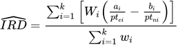
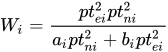
- where the weight, Wi, is the inverse of the estimated variance.
Pooled incidence rate ratio for fixed effects is estimated as follows:
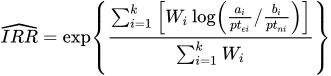
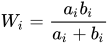
- where the weight, Wi, is the inverse of the estimated variance for the log transformed statistic.
Example
The example looks at mortality by sex and age for patients with trigeminal neuralgia (Rothman and Monson, 1973). The person-time data are person-years.
| Exposed | Not exposed | |||
| Group: | Cases | Person-time | Cases | Person-time |
| Age < 65: | 14 | 1516 | 10 | 1701 |
| Age >= 65: | 76 | 949 | 121 | 2245 |
To analyse these data in StatsDirect first prepare them in four workbook columns and label these columns appropriately. Alternatively, open the test workbook using the file open function of the file menu. Then select incidence rate difference from the meta-analysis section of the analysis menu. Select the columns marked "Exposed cases", "Exposed person-time", "Control cases" and "Control person-time" when prompted for data, and the column marked "Age split" for the stratum labels. Note that "exposed" and "experimental" groups are the same.
For this example:
Incidence rate difference (IRD) meta-analysis
| Stratum | Table (a, person-time exposed, b, person-time not exposed) | ||||
| 1 | 14 | 1516 | 10 | 1701 | Age < 65 |
| 2 | 76 | 949 | 121 | 2245 | Age >= 65 |
| Stratum | IRD | 95% CI (approximate) | ||
| 1 | 0.003356 | -0.0027 | 0.009412 | Age < 65 |
| 2 | 0.026187 | 0.005781 | 0.046593 | Age >= 65 |
| Stratum | Standardized effect | Variance | % Weights (fixed, random) | ||
| 1 | 0.003356 | 0.00001 | 91.904848 | 59.481911 | Age < 65 |
| 2 | 0.026187 | 0.000108 | 8.095152 | 40.518089 | Age >= 65 |
Fixed effects (inverse variance)
Pooled IRD = 0.005204 (95% CI = -0.000602 to 0.01101)
Z (test IRD differs from 0) = 1.756825 P = 0.0789
Non-combinability of studies
Cochran Q = 4.419452 (df = 1) P = 0.0355
Moment-based estimate of between studies variance = 0.000202
I² (inconsistency) = 77.4% (95% CI = 0% to 94.3%)
Random effects (DerSimonian-Laird)
Pooled IRD = 0.012607 (95% CI = -0.009361 to 0.034574)
Z (test IRD differs from 0) = 1.124754 P = 0.2607
Here we infer with 95% confidence, assuming a fixed effects model, that the true size of the difference between incidence rates was somewhere between -0.0006 and 0.011 deaths per person-year for the exposed group compared with the non-exposed group; i.e. not statistically significant.

 R code
This R code reproduces the example above, then runs the incidence rate ratio option on the same data. It needs no packages and was checked with R 4.6.1. Paste it into R, or save it as a script and run it.
# Incidence rate meta-analysis: the StatsDirect help example (Rothman and Monson 1973,
# deaths among patients with trigeminal neuralgia in two age strata, exposed and not
# exposed; the test workbook's meta worksheet columns Exposed cases, Exposed
# person-time, Control cases, Control person-time and Age split) in R
a <- c(14, 76)        # cases in the exposed groups
pt1 <- c(1516, 949)   # person-years in the exposed groups
b <- c(10, 121)       # cases in the non-exposed groups
pt2 <- c(1701, 2245)  # person-years in the non-exposed groups
strata <- c("Age < 65", "Age >= 65")
k <- length(a)
z <- qnorm(0.975)     # for 95% confidence intervals
six <- function(x) formatC(x, digits = 6, format = "f", drop0trailing = TRUE)
pv <- function(p) {
  if (p < 0.0001) "P < 0.0001" else
    paste("P =", formatC(p, digits = 4, format = "f", drop0trailing = TRUE))
}

# Base R has no meta-analysis function, so the pooling follows the formulae above: a
# fixed effects estimate weighted by inverse variance, Cochran's Q for heterogeneity,
# the DerSimonian-Laird moment estimate of the between-studies variance (tau squared,
# zero when Q is below its degrees of freedom) and the random effects estimate, whose
# weights add tau squared to each stratum's variance (two or more strata)
pool <- function(y, v) {
  w <- 1 / v
  fixed <- sum(w * y) / sum(w)
  q <- sum(w * (y - fixed)^2)
  tau2 <- max(0, (q - (k - 1)) / (sum(w) - sum(w^2) / sum(w)))
  wr <- 1 / (v + tau2)
  list(fixed = fixed, se = sqrt(1 / sum(w)), q = q, tau2 = tau2,
       random = sum(wr * y) / sum(wr), se_r = sqrt(1 / sum(wr)),
       fixed_pct = 100 * w / sum(w), random_pct = 100 * wr / sum(wr))
}
# The pooled part of the report; f back-transforms a log ratio to a ratio
summarise <- function(p, name, null, f = identity) {
  ci <- function(est, se) {
    paste0("(95% CI = ", six(f(est - z * se)), " to ", six(f(est + z * se)), ")")
  }
  cat("Fixed effects (inverse variance)\n")
  cat("Pooled", name, "=", six(f(p$fixed)), ci(p$fixed, p$se), "\n")
  cat("Z (test ", name, " differs from ", null, ") = ", six(p$fixed / p$se), "  ",
      pv(2 * pnorm(-abs(p$fixed / p$se))), "\n", sep = "")
  cat("Non-combinability of studies\n")
  cat("Cochran Q = ", six(p$q), "  (df = ", k - 1, ")  ",
      pv(pchisq(p$q, k - 1, lower.tail = FALSE)), "\n", sep = "")
  cat("Moment-based estimate of between studies variance =", six(p$tau2), "\n")
  # I2 is the share of Q beyond its degrees of freedom; StatsDirect adds a confidence
  # interval for it when there are at least three strata
  i2 <- max(0, 100 * (p$q - (k - 1)) / p$q)
  cat("I2 (inconsistency) = ",
      formatC(i2, digits = 1, format = "f", drop0trailing = TRUE), "%\n", sep = "")
  cat("Random effects (DerSimonian-Laird)\n")
  cat("Pooled", name, "=", six(f(p$random)), ci(p$random, p$se_r), "\n")
  cat("Z (test ", name, " differs from ", null, ") = ", six(p$random / p$se_r), "  ",
      pv(2 * pnorm(-abs(p$random / p$se_r))), "\n", sep = "")
}
# The forest plots that follow in the report: each stratum's estimate and interval, a
# box that grows with its weight, and the pooled estimate as a diamond at the foot
forest <- function(est, lower, upper, pooled, p_lower, p_upper, pct, main, xlab,
                   null, log = "") {
  par(mar = c(5, 7, 4, 2))
  y <- (k + 1):2
  plot(NA, xlim = range(lower, upper, p_lower, p_upper), ylim = c(0.5, k + 1.5),
       log = log, yaxt = "n", ylab = "", xlab = xlab, main = main)
  axis(2, at = c(y, 1), labels = c(strata, "combined"), las = 1, tick = FALSE)
  abline(v = null, lty = 3)
  segments(lower, y, upper, y)
  points(est, y, pch = 15, cex = 0.5 + 2 * sqrt(pct / 100))
  polygon(c(p_lower, pooled, p_upper, pooled), c(1, 1.2, 1, 0.8), col = "grey")
}

# Each stratum's incidence rate difference, with its approximate interval: the
# difference plus and minus z standard errors, from the Poisson variance of the
# difference, a/pt1^2 + b/pt2^2, which the fixed effects weights invert
ird <- a / pt1 - b / pt2
v_ird <- a / pt1^2 + b / pt2^2
se_ird <- sqrt(v_ird)
res <- pool(ird, v_ird)
cat("Incidence rate difference (IRD) meta-analysis\n")
print(data.frame(stratum = 1:k, IRD = six(ird), lower = six(ird - z * se_ird),
                 upper = six(ird + z * se_ird), strata), row.names = FALSE)
# The report's next table: the standardised effect is the difference itself, with its
# variance beside the weights
print(data.frame(stratum = 1:k, effect = six(ird), variance = six(v_ird),
                 fixed = six(res$fixed_pct), random = six(res$random_pct), strata),
      row.names = FALSE)
summarise(res, "IRD", 0)
forest(ird, ird - z * se_ird, ird + z * se_ird, res$fixed, res$fixed - z * res$se,
       res$fixed + z * res$se, res$fixed_pct,
       "Incidence rate difference meta-analysis plot [fixed effects]",
       "incidence rate difference (95% confidence interval)", 0)
forest(ird, ird - z * se_ird, ird + z * se_ird, res$random, res$random - z * res$se_r,
       res$random + z * res$se_r, res$random_pct,
       "Incidence rate difference meta-analysis plot [random effects]",
       "incidence rate difference (95% confidence interval)", 0)

# The same data as incidence rate ratios, StatsDirect's other option for this menu
# item. poisson.test compares two rates and gives their ratio with the exact interval
# of the report, from the binomial distribution of the exposed cases among all cases.
# The standardised effect is the log ratio and the fixed effects weights invert its
# variance, 1/a + 1/b
irr <- (a / pt1) / (b / pt2)
exact <- sapply(1:k, function(i) {
  poisson.test(c(a[i], b[i]), c(pt1[i], pt2[i]))$conf.int
})
res_r <- pool(log(irr), 1 / a + 1 / b)
cat("Incidence rate ratio (IRR) meta-analysis\n")
print(data.frame(stratum = 1:k, IRR = six(irr), lower = six(exact[1, ]),
                 upper = six(exact[2, ]), strata), row.names = FALSE)
print(data.frame(stratum = 1:k, effect = six(log(irr)),
                 variance = six(1 / a + 1 / b),
                 fixed = six(res_r$fixed_pct), random = six(res_r$random_pct), strata),
      row.names = FALSE)
summarise(res_r, "IRR", 1, exp)

# The report's exact conditional block (Martin and Austin 2000): given a stratum's
# total cases, its exposed cases are binomial with probability pt1 psi / (pt1 psi + pt2)
# for a common rate ratio psi, so the total of exposed cases over the strata has
# the convolution of these binomials as its conditional distribution. Under psi = 1
# each is dbinom(x, a + b, pt1 / (pt1 + pt2)); another psi multiplies the probability of
# x exposed cases by psi^x. The conditional maximum likelihood estimate is the psi
# whose expected total equals the observed total, and each exact limit the psi at
# which one tail probability of the observed total is 2.5% (the mid-P versions count
# half of the observed total's probability). The P values are the tails at psi = 1,
# the two sided Fisher P summing the outcomes no more probable than the observed one
null_p <- 1
for (i in 1:k) {
  coef <- dbinom(0:(a[i] + b[i]), a[i] + b[i], pt1[i] / (pt1[i] + pt2[i]))
  product <- numeric(length(null_p) + length(coef) - 1)
  for (j in seq_along(coef)) {
    at <- j:(j + length(null_p) - 1)
    product[at] <- product[at] + coef[j] * null_p
  }
  null_p <- product
}
x <- seq_along(null_p) - 1
s <- sum(a)
cond <- function(psi) {
  lp <- log(null_p) + x * log(psi)
  p <- exp(lp - max(lp))
  p / sum(p)
}
tail_p <- function(psi, upper, half = 1) {
  p <- cond(psi)
  sum(p[if (upper) x > s else x < s]) + half * p[x == s]
}
root <- function(f) uniroot(f, c(0.01, 100), tol = 1e-10)$root  # brackets this example
cmle <- root(function(psi) sum(x * cond(psi)) - s)
fisher <- c(root(function(psi) tail_p(psi, TRUE) - 0.025),
            root(function(psi) tail_p(psi, FALSE) - 0.025))
mid <- c(root(function(psi) tail_p(psi, TRUE, 0.5) - 0.025),
         root(function(psi) tail_p(psi, FALSE, 0.5) - 0.025))
p_null <- cond(1)
one_f <- min(tail_p(1, TRUE), tail_p(1, FALSE))
two_f <- sum(p_null[p_null <= p_null[x == s]])
one_m <- min(tail_p(1, TRUE, 0.5), tail_p(1, FALSE, 0.5))
cat("Fixed effects (conditional maximum likelihood)\n")
cat("Pooled rate ratio =", six(cmle), "\n")
cat("Exact Fisher 95% confidence interval =", six(fisher[1]), "to", six(fisher[2]),
    "\n")
cat("Exact Fisher one sided ", pv(one_f), ", two sided ", pv(two_f), "\n", sep = "")
cat("Exact mid-P 95% confidence interval =", six(mid[1]), "to", six(mid[2]), "\n")
cat("Exact mid-P one sided ", pv(one_m), ", two sided ", pv(min(1, 2 * one_m)), "\n",
    sep = "")
forest(irr, exact[1, ], exact[2, ], exp(res_r$fixed), exp(res_r$fixed - z * res_r$se),
       exp(res_r$fixed + z * res_r$se), res_r$fixed_pct,
       "Incidence rate ratio meta-analysis plot [fixed effects]",
       "incidence rate ratio (95% confidence interval)", 1, log = "x")
forest(irr, exact[1, ], exact[2, ], exp(res_r$random),
       exp(res_r$random - z * res_r$se_r), exp(res_r$random + z * res_r$se_r),
       res_r$random_pct, "Incidence rate ratio meta-analysis plot [random effects]",
       "incidence rate ratio (95% confidence interval)", 1, log = "x")