Effect Size Meta-analysis
Menu location: Analysis_Meta-Analysis_Effect Size.
Case-control studies of continuous outcomes (e.g. serum creatinine) may be investigated with respect to overall size of effect of an intervention. Meta-analysis may be used to investigate the combination or interaction of a group of independent studies, for example a series of effect sizes from similar studies conducted at different centres. This StatsDirect function examines the effect size within each stratum and across all of the studies/strata.
There are a number of statistical methods for estimating effect size, StatsDirect uses g (modified Glass statistic with pooled sample standard deviation) and the unbiased estimator d (Hedges and Olkin, 1985):
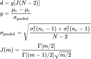
- where ne is the number in the experimental group, nc is the number in the control group, μe is the sample mean of the experimental group, μc is the sample mean of the control group, σe is the sample standard deviation for the experimental group, σc is the sample standard deviation for the control group, N = ne + nc, J(m) is the correction factor given m and Γ is the gamma function.
For each study StatsDirect gives g with an exact confidence interval and d with an approximate confidence interval. An iterative method based on the non-central t distribution is used to construct the confidence interval for g (Hedges and Olkin, 1985).
The pooled mean effect size estimate (d+) is calculated using direct weights defined as the inverse of the variance of d for each study/stratum. An approximate confidence interval for d+ is given with a z statistic and probability of this pooled effect size being equal to zero (Hedges and Olkin, 1985).
StatsDirect also gives the option to base effect size calculations on weighted mean difference (a non-standardized estimate unlike g and d) as described in the Cochrane Collaboration Handbook (Mulrow and Oxman, 1996). The confidence interval for the mean difference of each study is calculated from the variances of its two groups taken separately, as the weights are.
The inconsistency of results across studies is summarised in the I² statistic, which is the percentage of variation across studies that is due to heterogeneity rather than chance – see the heterogeneity section for more information.
Please note that the results from StatsDirect may be slightly different from the results you obtain using other packages or from those quoted in papers; this is due to the use of exact bias correction calculated from the gamma distribution in StatsDirect.
DATA INPUT:
You may enter number, mean and standard deviation for control and experimental groups of each study. Alternatively you may just enter numbers in experimental groups, numbers in control groups and effect size g (nb. please make sure you use g only as defined above!).
Example
From personal communication from Dr N. Freemantle.
The following data represent test outcomes for six studies in which an educational intervention was investigated:
| Experimental | Control | |||||
| Trial | N | Mean | SD | N | Mean | SD |
| Kottke | 27 | 18.50 | 14.90 | 17 | 5.40 | 17.30 |
| Levinson | 16 | 60.00 | 29.20 | 15 | 55.00 | 29.20 |
| Oliver (intensive) | 25 | 10.72 | 6.46 | 66 | 6.92 | 6.83 |
| Oliver (standard) | 62 | 9.20 | 6.16 | 66 | 6.92 | 6.83 |
| Sulmasy | 9 | 3.75 | 2.55 | 22 | 1.05 | 2.12 |
| White | 63 | 60.00 | 13.30 | 40 | 46.30 | 18.60 |
| Wilson | 23 | 9.24 | 5.35 | 23 | 5.33 | 4.48 |
To analyse these data in StatsDirect first prepare them in seven workbook columns and label these columns appropriately. Alternatively, open the test workbook using the file open function of the file menu. Then select effect size from the meta-analysis section of the analysis menu, select the option to use mean, n and sd, and then select the columns ’Exptal. number’, ’Exptal. mean’, ’Exptal. SD’, ’Control number’, ’Control mean’, ’Control SD’ and ’Trial’ as prompted.
For this example:
| Study | J(N-2) | g | Exact 95% CI | ||
| 1 | 0.982018 | 0.826124 | 0.189712 | 1.453464 | Kottke |
| 2 | 0.973875 | 0.171233 | -0.536003 | 0.87554 | Levinson |
| 3 | 0.991545 | 0.564449 | 0.09524 | 1.030587 | Oliver (intensive) |
| 4 | 0.994034 | 0.350002 | -0.000005 | 0.698642 | Oliver (standard) |
| 5 | 0.973875 | 1.20168 | 0.358317 | 2.027136 | Sulmasy |
| 6 | 0.992553 | 0.880352 | 0.46397 | 1.292737 | White |
| 7 | 0.982841 | 0.792426 | 0.187185 | 1.38934 | Wilson |
| Study | N (exptal.) | N (control) | d | Approximate 95% CI | ||
| 1 | 27 | 17 | 0.811269 | 0.18121 | 1.441328 | Kottke |
| 2 | 16 | 15 | 0.166759 | -0.538869 | 0.872388 | Levinson |
| 3 | 25 | 66 | 0.559677 | 0.092265 | 1.027089 | Oliver (intensive) |
| 4 | 62 | 66 | 0.347914 | -0.001341 | 0.697169 | Oliver (standard) |
| 5 | 9 | 22 | 1.170286 | 0.341855 | 1.998716 | Sulmasy |
| 6 | 63 | 40 | 0.873796 | 0.459972 | 1.28762 | White |
| 7 | 23 | 23 | 0.778829 | 0.179356 | 1.378302 | Wilson |
| Study | % weights (fixed, random) | ||
| 1 | 9.19968 | 10.62611 | Kottke |
| 2 | 7.334723 | 8.764878 | Levinson |
| 3 | 16.716159 | 17.01627 | Oliver (intensive) |
| 4 | 29.939856 | 25.212518 | Oliver (standard) |
| 5 | 5.321368 | 6.605485 | Sulmasy |
| 6 | 21.325794 | 20.235667 | White |
| 7 | 10.162419 | 11.53907 | Wilson |
Fixed effects (Hedges-Olkin)
Pooled effect size d+ = 0.612354 (95% CI = 0.421251 to 0.803457)
Z (test d+ differs from 0) = 6.280333 P < 0.0001
Non-combinability of studies
Cochran Q = 7.737692 (df = 6) P = 0.258
Moment-based estimate of between studies variance = 0.020397
I² (inconsistency) = 22.5% (95% CI = 0% to 72.5%)
Random effects (DerSimonian-Laird)
Pooled d+ = 0.627768 (95% CI = 0.403026 to 0.85251)
Z (test d+ differs from 0) = 5.474734 P < 0.0001
Bias indicators
Begg-Mazumdar: Kendall's tau = 0.238095 P = 0.5619 (low power)
Egger: bias = 1.439076 (90% CI = -1.712135 to 4.590287) P = 0.3997
Here we can say with 95% confidence, assuming a random effects model, that the true size of the effect was at least 0.4 greater for the group who received the educational intervention compared with those who did not. Assuming a fixed effects model a slightly stronger inference could be made about an effect size of 0.42 (the lower confidence limit) but the high inter-study variation makes the fixed effects model less appropriate.

 R code
This R code reproduces the example above. It needs no packages and was checked with R 4.6.1. Paste it into R, or save it as a script and run it.
# Effect size meta-analysis: the StatsDirect help example (Freemantle, personal
# communication, test outcomes of seven comparisons from six trials of an educational
# intervention; the test workbook's meta worksheet columns J to P) in R
trial <- c("Kottke", "Levinson", "Oliver (intensive)", "Oliver (standard)", "Sulmasy",
           "White", "Wilson")
en <- c(27, 16, 25, 62, 9, 63, 23)
em <- c(18.5, 60, 10.72, 9.2, 3.75, 60, 9.24)
es <- c(14.9, 29.2, 6.46, 6.16, 2.55, 13.3, 5.35)
cn <- c(17, 15, 66, 66, 22, 40, 23)
cm <- c(5.4, 55, 6.92, 6.92, 1.05, 46.3, 5.33)
cs <- c(17.3, 29.2, 6.83, 6.83, 2.12, 18.6, 4.48)
k <- length(en)

# Base R has no meta-analysis function, so the statistics are computed as the
# formulae above give them. g is the difference in means over the pooled standard
# deviation; d is g corrected for its small sample bias by J(N - 2), computed from
# the gamma function (lgamma is its logarithm), or from the usual approximation
# 1 - 3 / (4m - 1) when N - 2 is 200 or more
six <- function(x) formatC(x, digits = 6, format = "f", drop0trailing = TRUE)
pv <- function(p) {
  if (p < 0.0001) "P < 0.0001" else
    paste("P =", formatC(p, digits = 4, format = "f", drop0trailing = TRUE))
}
n <- en + cn
m <- n - 2
s <- sqrt(((en - 1) * es^2 + (cn - 1) * cs^2) / m)
g <- (em - cm) / s
J <- ifelse(m < 200, exp(lgamma(m / 2) - lgamma((m - 1) / 2)) / sqrt(m / 2),
            1 - 3 / (4 * m - 1))
d <- J * g
z <- qnorm(0.975)

# The approximate confidence interval for d uses its large sample variance. The
# exact interval for g comes from the noncentral t distribution: g times
# sqrt(ne * nc / N) is a t statistic on N - 2 degrees of freedom whose
# noncentrality parameter is the true effect size times the same factor, so each
# limit is the noncentrality parameter that puts the observed statistic at the
# 97.5th or the 2.5th percentile, found with uniroot and pt. R's pt is accurate
# for noncentrality parameters up to 37.62 (see its help page); here the largest is
# under 5, so a guard is only needed for a very large trial with a large effect
vard <- n / (en * cn) + d^2 / (2 * n)
lcid <- d - z * sqrt(vard)
ucid <- d + z * sqrt(vard)
scale <- sqrt(en * cn / n)
ncp_limit <- function(t, df, hw, p) {
  f <- function(nc) pt(t, df, ncp = nc) - p
  uniroot(f, if (p > 0.5) c(t - 2 * hw, t) else c(t, t + 2 * hw), tol = 1e-10)$root
}
hw <- z * sqrt(vard) * scale
lcig <- mapply(ncp_limit, g * scale, m, hw, 0.975) / scale
ucig <- mapply(ncp_limit, g * scale, m, hw, 0.025) / scale
print(data.frame(trial, J = six(J), g = six(g), exact_lower = six(lcig),
                 exact_upper = six(ucig)), row.names = FALSE)
print(data.frame(trial, en, cn, d = six(d), approx_lower = six(lcid),
                 approx_upper = six(ucid)), row.names = FALSE)

# Fixed effects (Hedges-Olkin): d weighted by the inverse of its variance
w <- 1 / vard
dplus <- sum(w * d) / sum(w)
se_dplus <- sqrt(1 / sum(w))
cat("Fixed effects (Hedges-Olkin)\n")
cat("Pooled effect size d+ = ", six(dplus), " (95% CI = ", six(dplus - z * se_dplus),
    " to ", six(dplus + z * se_dplus), ")\n", sep = "")
cat("Z (test d+ differs from 0) =", six(dplus / se_dplus), " ",
    pv(2 * pnorm(-abs(dplus / se_dplus))), "\n")

# Heterogeneity: Cochran's Q, the DerSimonian-Laird moment estimate of the between
# studies variance and I-squared. The interval for I-squared is the iterative
# noncentral chi-square method of Hedges and Pigott (2001): Q is taken as a
# noncentral chi-square variable on df degrees of freedom, and each limit is the
# noncentrality parameter lambda that puts the observed Q at its 97.5th or 2.5th
# percentile (found with uniroot and pchisq; 0 when the central distribution already
# puts Q below that percentile), converted to I-squared as 100 lambda / (df + lambda)
Q <- sum(w * (d - dplus)^2)
df <- k - 1
tausq <- max(0, (Q - df) / (sum(w) - sum(w^2) / sum(w)))
isq <- max(0, 100 * (Q - df) / Q)
ncp_chisq <- function(p) {
  if (pchisq(Q, df) < p) return(0)
  uniroot(function(lambda) pchisq(Q, df, ncp = lambda) - p, c(0, 10 * Q + 100),
          tol = 1e-10)$root
}
lambda_ci <- c(ncp_chisq(0.975), ncp_chisq(0.025))
isq_ci <- 100 * lambda_ci / (df + lambda_ci)
pc1 <- function(x) formatC(x, digits = 1, format = "f", drop0trailing = TRUE)
cat("Non-combinability of studies\n")
cat("Cochran Q = ", six(Q), "  (df = ", df, ")  ",
    pv(pchisq(Q, df, lower.tail = FALSE)), "\n", sep = "")
cat("Moment-based estimate of between studies variance =", six(tausq), "\n")
cat("I-squared (inconsistency) = ", pc1(isq), "% (95% CI = ", pc1(isq_ci[1]), "% to ",
    pc1(isq_ci[2]), "%)\n", sep = "")

# Random effects (DerSimonian-Laird): the between studies variance is added to
# each study's variance before weighting
wr <- 1 / (vard + tausq)
dsd <- sum(wr * d) / sum(wr)
se_dsd <- sqrt(1 / sum(wr))
cat("Random effects (DerSimonian-Laird)\n")
cat("Pooled d+ = ", six(dsd), " (95% CI = ", six(dsd - z * se_dsd), " to ",
    six(dsd + z * se_dsd), ")\n", sep = "")
cat("Z (test d+ differs from 0) =", six(dsd / se_dsd), " ",
    pv(2 * pnorm(-abs(dsd / se_dsd))), "\n")
cat("% weights (fixed, random)\n")
print(data.frame(trial, fixed = six(100 * w / sum(w)),
                 random = six(100 * wr / sum(wr))), row.names = FALSE)

# Bias indicators. Begg and Mazumdar's test is Kendall's rank correlation between
# each study's standardised deviation from the pooled effect and its variance,
# with the exact P value; cor.test computes it by default only for fewer than 50
# studies, so exact = TRUE asks for it whatever their number (with tied ranks the
# program uses tau-b with a normal approximation and a continuity correction instead).
# The report notes the test's low power with fewer than eleven studies. Egger's test
# regresses the standard normal deviate d / se on the precision 1 / se: the
# intercept estimates the bias, judged here with a 90% interval on k - 2 degrees
# of freedom
se <- sqrt(vard)
ts <- (d - dplus) / sqrt(vard - 1 / sum(w))
begg <- cor.test(ts, vard, method = "kendall", exact = TRUE)
power_note <- if (k < 11) "(low power)" else ""
cat("Bias indicators\n")
cat("Begg-Mazumdar: Kendall's tau =", six(begg$estimate), " ", pv(begg$p.value),
    power_note, "\n")
egger <- lm(I(d / se) ~ I(1 / se))
bias <- coef(summary(egger))[1, ]
cat("Egger: bias = ", six(bias["Estimate"]), " (90% CI = ",
    six(bias["Estimate"] - qt(0.95, k - 2) * bias["Std. Error"]), " to ",
    six(bias["Estimate"] + qt(0.95, k - 2) * bias["Std. Error"]), ")  ",
    pv(bias["Pr(>|t|)"]), "\n", sep = "")

# The bias assessment plot that follows in the report: each study's d against its
# standard error, with the smallest standard errors at the top, the fixed effects
# pooled d+ as a vertical line and the 95% limits expected around it as a funnel
plot(d, se, ylim = rev(range(0, se)), xlim = range(lcid, ucid), pch = 1,
     xlab = "Effect size", ylab = "Standard error", main = "Bias assessment plot")
abline(v = dplus)
se_line <- seq(0, max(se), length.out = 100)
lines(dplus + z * se_line, se_line)
lines(dplus - z * se_line, se_line)

# The forest plots: each study's d with its approximate 95% interval and a square
# proportional to its size, then the pooled estimate as a diamond, for the fixed
# and the random effects models (the program prefixes the random effects label
# with DL for DerSimonian-Laird)
forest <- function(pooled, lower, upper, label) {
  y <- k:1 + 1
  plot(d, y, xlim = range(lcid, ucid, lower, upper), ylim = c(0.5, k + 1.5),
       yaxt = "n", ylab = "", xlab = "", main = label, pch = 15,
       cex = 1 + 2 * n / max(n))
  axis(2, at = c(y, 1), labels = c(trial, "pooled"), las = 1, tick = FALSE)
  segments(lcid, y, ucid, y)
  polygon(c(lower, pooled, upper, pooled), c(1, 1.25, 1, 0.75))
  abline(v = pooled, lty = 2)
  if (min(lcid) < 0) abline(v = 0)
  prefix <- if (grepl("random", label)) "DL " else ""
  mtext(paste0(prefix, "pooled effect size = ", six(pooled), "  (95% CI = ",
               six(lower), " to ", six(upper), ")"), side = 3, line = 0.3, cex = 0.9)
}
op <- par(mar = c(3, 9, 4, 1))
forest(dplus, dplus - z * se_dplus, dplus + z * se_dplus,
       "Effect size meta-analysis plot [fixed effects]")
forest(dsd, dsd - z * se_dsd, dsd + z * se_dsd,
       "Effect size meta-analysis plot [random effects]")
par(op)