Spearman's Rho and Hotelling-Pabst T distribution
Menu location: Analysis_Distributions_Spearman's rho.
Given a value for the Hotelling-Pabst test statistic (T) or Spearman's rho (ρ) this function calculates the upper tail probability: that of obtaining a rank correlation at least as large as the one given, which is a value of T less than or equal to the T given.
For two rankings (x1,x2...xn and y1,y2...yn) of n objects without ties:
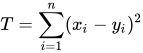
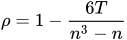
T is related to the Spearman rank correlation coefficient (ρ) by:
Technical Validation
Probabilities are calculated by summation across all permutations when n is 10 or fewer and by an Edgeworth series approximation when n > 10 (Best and Roberts, 1975). The exact calculation employs a corrected version of the Best and Roberts (1975) algorithm. The Edgeworth series results for n > 10 are within 0.0004 of the exact probabilities at n = 11 and within 0.00005 by n = 15; the approximation improves as n grows.
The inverse is calculated by finding the largest value of T that gives a calculated probability (using the method above) closest to but not greater than the P value entered.
Illustration
Consider the ten pairs of rankings in the Spearman rank correlation example, a tutor's rankings of ten students for suitability to their career and for knowledge of psychology. The sum of the squared differences between the paired ranks is T = 52, so ρ = 1 - 6 × 52/990 = 0.684848. To calculate the probability of a rank correlation at least this large when the two rankings are independent, select Spearman's rho from the Distributions section of the Analysis menu, enter 10 as the sample size and 52 as Hotelling-Pabst T (or enter 0.684848 as Spearman's rho, from which StatsDirect calculates T) and click Calculate. StatsDirect shows the upper tail probability, that of a T no larger than 52, and reports it as:
P(Hotelling T 52, n 10) = 0.017325837742504 upper tail
Of the 10! = 3,628,800 equally likely orderings of one ranking against the other, 62,872 give a T of 52 or less. This is the upper side P of the exact test in the Spearman rank correlation report (P = 0.0173); the distribution of ρ is symmetrical about zero, so the two sided P is twice it (P = 0.0347).
For the inverse, enter 10 as the sample size and 0.025 as the upper tail P and click Invert. StatsDirect finds the largest T whose upper tail probability does not exceed 0.025, shows it with its rho (T = 58, ρ = 0.648484848484848) and reports the probability that it cuts off:
Hotelling T (upper tail P 0.025, n 10) = 0.02448936287478
So with ten pairs a rho of 0.648485 or more (a T of 58 or less) is significant at the one sided 2.5% level, as the example's 0.684848 is. The next possible value, T = 60 (ρ = 0.636364), has an upper tail probability of 0.027215332892416 and is not: with so few pairs the attainable significance levels are coarse.
With more than ten pairs the probability comes from the Edgeworth series. Enter 20 as the sample size and 0.4 as Spearman's rho: StatsDirect calculates T = 798 and reports:
P(Hotelling T 798, n 20) = 0.040820092284141 upper tail
The probabilities in this illustration were calculated in R with the code below; StatsDirect displays them to 15 decimal places.

 R code
This R code reproduces the illustration above. It needs no packages and was checked with R 4.6.1. Paste it into R, or save it as a script and run it.
# Spearman's rho distribution: the StatsDirect help illustration (T = 52 for the 10
# pairs of rankings of the Spearman rank correlation example, Armitage and Berry 1994,
# p. 466, the test workbook's Nonparametric worksheet columns Career and Psychology;
# the T that cuts off an upper tail of 0.025; and rho = 0.4 for 20 pairs) in R
career <- c(4, 10, 3, 1, 9, 2, 6, 7, 8, 5)
psychology <- c(5, 8, 6, 2, 10, 3, 9, 4, 7, 1)
n <- length(career)                       # 10 pairs

fifteen <- function(x) formatC(x, digits = 15, format = "f", drop0trailing = TRUE)
six <- function(x) formatC(x, digits = 6, format = "f", drop0trailing = TRUE)
pv <- function(p) {
  if (p < 0.0001) "P < 0.0001" else paste("P =", formatC(p, digits = 4, format = "f"))
}

# The Hotelling-Pabst statistic T is the sum of the squared differences between the
# paired ranks (Spearman's score in the StatsDirect rank correlation report), and rho
# follows from it: rho = 1 - 6T/(n^3 - n)
score <- sum((career - psychology)^2)
rho <- 1 - 6 * score / (n^3 - n)
cat("T =", score, " Spearman's rho =", fifteen(rho), "\n")

# The distribution of T for n pairs ranked without ties when the two rankings are
# independent: each of the n! orderings of one ranking against the other is equally
# likely. For n = 5 all 120 orderings can be listed and T found for each
perms <- function(m) {
  if (m == 1) return(matrix(1))
  p <- perms(m - 1)
  do.call(rbind, lapply(1:m, function(i) cbind(i, p + (p >= i))))
}
t5 <- rowSums((perms(5) - rep(1:5, each = 120))^2)
print(table(t5))                          # T is even, from 0 to 40

# Listing the orderings is impractical for larger n (10! is 3,628,800), but the counts
# of orderings by T can be built up one position at a time: for each set of ranks
# already placed in the first positions, keep the counts of the partial orderings by
# their sum of squared differences so far; placing rank r at position i adds (i - r)^2
counts_by_T <- function(n) {
  top <- n * (n^2 - 1) / 3                # the largest T, for the reversed ranking
  counts <- vector("list", 2^n)           # one entry per set of ranks placed
  counts[[1]] <- c(1, numeric(top))       # nothing placed: one ordering with T = 0
  bit <- 2^(0:(n - 1))
  for (set in 0:(2^n - 2)) {
    so_far <- counts[[set + 1]]
    if (is.null(so_far)) next
    i <- sum(bitwAnd(set, bit) > 0) + 1   # the next position to fill
    for (r in (1:n)[bitwAnd(set, bit) == 0]) {
      added <- c(numeric((i - r)^2), so_far)[seq_len(top + 1)]
      to <- set + bit[r] + 1
      counts[[to]] <- if (is.null(counts[[to]])) added else counts[[to]] + added
    }
  }
  counts[[2^n]]                           # counts for T = 0, 1, ..., top
}
stopifnot(all(tabulate(t5 + 1, nbins = 41) == counts_by_T(5)))
upper <- function(t, n) {                 # P(T <= t): the upper tail probability of rho
  counts <- counts_by_T(n)
  sum(counts[seq_len(t + 1)]) / sum(counts)
}
counts <- counts_by_T(n)
at_most_T <- sum(counts[seq_len(score + 1)])
cat(format(at_most_T, big.mark = ","), "of the", format(sum(counts), big.mark = ","),
    "orderings give T of", score, "or less\n")

# The line the StatsDirect dialog reports for T = 52 with 10 pairs, to 15 decimal
# places: the probability of a rank correlation at least as large as 0.684848, which
# is a T no larger than 52
cat("P(Hotelling T ", score, ", n ", n, ") = ", fifteen(upper(score, n)),
    " upper tail\n", sep = "")
# This is the upper side P of the exact test in the Spearman rank correlation report;
# the distribution of rho is symmetrical about 0, so the two sided P is twice it
cat("Upper side", pv(upper(score, n)), "\n")
cat("Two sided", pv(2 * upper(score, n)), "\n")
# cor.test(career, psychology, method = "spearman", alternative = "greater") gives the
# same S = 52 and rho, but its P here is 0.0175, from a series approximation: its P for
# Spearman's rho is exact only with fewer than 10 pairs (see the 20 pairs below)

# The inverse: the largest T whose upper tail probability does not exceed the P
# entered, here 0.025 for 10 pairs. StatsDirect shows that T and its rho, and reports
# the probability it actually cuts off
critical <- function(P, n) {
  counts <- counts_by_T(n)
  tail <- cumsum(counts) / sum(counts)    # P(T <= t) for t = 0, 1, ..., top
  t <- seq(0, length(counts) - 1, by = 2) # the possible values of T are even
  max(t[tail[t + 1] <= P])
}
k <- critical(0.025, n)
rho_k <- 1 - 6 * k / (n^3 - n)
cat("T =", k, "  Spearman's rho =", fifteen(rho_k), "\n")
cat("Hotelling T (upper tail P 0.025, n ", n, ") = ", fifteen(upper(k, n)), "\n",
    sep = "")
cat("So a rho of", six(rho_k), "or more (a T of", k, "or less) is significant at the",
    "one sided 2.5% level\n")
# The next possible T cuts off more than 0.025, so its rho is not significant
cat("T = ", k + 2, " (rho = ", six(1 - 6 * (k + 2) / (n^3 - n)), "): P(Hotelling T ",
    k + 2, ", n ", n, ") = ", fifteen(upper(k + 2, n)), " upper tail\n", sep = "")

# For more than 10 pairs StatsDirect uses an Edgeworth series (Best and Roberts 1975),
# as cor.test does for 10 or more pairs, so for 20 pairs the two agree. Entering rho =
# 0.4 in StatsDirect gives T = (1 - 0.4) * 20 * (20^2 - 1) / 6 = 798; in R the series
# is reached through cor.test on two rankings with that T, here 1 to 20 against the
# same ranks with four pairs of positions swapped (swapping positions i and j adds
# 2 * (i - j)^2 to T: 2 * (361 + 36 + 1 + 1) = 798)
x <- 1:20
y <- x
y[c(1, 20)] <- y[c(20, 1)]
y[c(2, 8)] <- y[c(8, 2)]
y[c(3, 4)] <- y[c(4, 3)]
y[c(5, 6)] <- y[c(6, 5)]
score20 <- sum((x - y)^2)
cat("T =", score20, " Spearman's rho =", fifteen(1 - 6 * score20 / (20^3 - 20)), "\n")
print(cor.test(x, y, method = "spearman", alternative = "greater"))
p20 <- cor.test(x, y, method = "spearman", alternative = "greater")$p.value
cat("P(Hotelling T ", score20, ", n 20) = ", fifteen(p20), " upper tail\n", sep = "")