Non-central t Distribution

Menu location: Analysis_Distributions_Non-Central t.

Non-central t (T) represents a family of distributions which are shaped by ν degrees of freedom and a non-centrality parameter (δ).

Non-central t may be expressed in terms of a normal and a chi-square distribution:

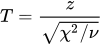
- where z is a normal variable with mean δ and variance 1 and χ² is a chi-square random variable with ν degrees of freedom (Owen, 1965).

In the field of meta-analysis some effect size statistics display a non-central t distribution. This function may therefore be useful in hypothesis testing and confidence interval construction for effect sizes (Greenland and Robins, 1985).

Technical Validation

StatsDirect evaluates the cumulative probability that a t random variable is less than or equal to a given value of T with n degrees of freedom and non-centrality parameter δ (Lenth, 1989; Owen, 1965; Young and Minder, 1974; Thomas, 1979; Chou, 1985; Boys 1989; Goedhart and Jansen, 1992). The inverse of T is found by conventional root finding methods to the precision shown.

Illustration

Select Non-Central t from the Distributions section of the Analysis menu. Enter a value of t, its degrees of freedom (a whole number) and the non-centrality parameter, then press Calculate to see the probability that a non-central t random variable is at or below that value (P for t <= t, the lower tail) and the probability that it is above it (P for t > t, the upper tail). Alternatively enter a lower tail probability with the degrees of freedom and non-centrality, then press Invert to see the value of t that has that probability below it; the report labels that line with the upper tail probability.

For example:

P(non-central t < 2.5, df 10, delta 1) = 0.103454395602356 upper, 0.896545604397644 lower

non-central t(P 0.1, df 10, delta 1) = 2.52607989706019

A non-central t with 10 degrees of freedom and non-centrality 1 falls below 2.5 with probability 0.8965, and below 2.526080 with probability 0.9.

The power of a t test comes from this distribution. A paired or single sample t test on 20 observations at the two sided 5% level rejects when the absolute value of t exceeds 2.093024, the critical value of Student's t on 19 degrees of freedom. If the true mean difference is half a standard deviation, t follows a non-central t distribution with 19 degrees of freedom and non-centrality 0.5 × √20 = 2.236068, so:

P(non-central t < 2.093024, df 19, delta 2.236068) = 0.564482925241891 upper, 0.435517074758109 lower

P(non-central t < -2.093024, df 19, delta 2.236068) = 0.999978478237757 upper, 0.000021521762243 lower

The power of the test is the probability of exceeding 2.093024, 0.5644829, plus the probability of falling below -2.093024, 0.0000215: in all 0.5645044 (R's power.t.test gives power = 0.5645044 from the unrounded critical value). Twenty observations give only a 56% chance of detecting a difference of half a standard deviation at the 5% level. These are the values StatsDirect gives: direct numerical integration of the distribution confirms them to the precision shown, and R's pt and qt (see the R code below) agree with them to 12 decimal places.

R code

This R code reproduces the illustration above to 12 decimal places (R's non-central t functions are accurate to about that many places here; StatsDirect shows up to 15 decimal places). It needs no packages and was checked with R 4.6.1. Paste it into R, or save it as a script and run it.

# Non-central t distribution: the illustration in the StatsDirect help (a tail
# probability, its inverse, and the power of a t test, as the Distributions dialog
# computes them) in R
# StatsDirect shows these to up to 15 decimal places. R's pt evaluates the non-central t
# distribution by the series of Lenth (1989) and qt inverts it (see the help for pt);
# here they agree with StatsDirect's values to 12 decimal places, so 12 are printed.
twelve <- function(x) formatC(x, digits = 12, format = "f", drop0trailing = TRUE)
seven <- function(x) formatC(x, digits = 7, format = "f", drop0trailing = TRUE)

# Tail probabilities of t = 2.5 on 10 degrees of freedom with non-centrality 1:
# pt(q, df, ncp) is the lower tail (P for t <= t); lower.tail = FALSE gives the upper
cat("P(non-central t < 2.5, df 10, delta 1) =",
    twelve(pt(2.5, 10, ncp = 1, lower.tail = FALSE)), "upper,",
    twelve(pt(2.5, 10, ncp = 1)), "lower\n")

# The inverse: the value of t below which the distribution has probability 0.9 (Invert
# with 0.9 as P for t <= t; the report labels the line with the upper tail, 0.1)
cat("non-central t(P 0.1, df 10, delta 1) =", twelve(qt(0.9, 10, ncp = 1)), "\n")

# Power of a paired or single sample t test on n = 20 observations at the two sided 5%
# level when the true mean difference is d = 0.5 standard deviations: under that
# alternative t has 19 degrees of freedom and non-centrality d * sqrt(n). The critical
# value and the non-centrality are rounded to the 6 places typed into the dialog.
n <- 20
d <- 0.5
delta <- round(d * sqrt(n), 6)              # 2.236068
crit <- round(qt(0.975, n - 1), 6)          # 2.093024
upper <- pt(crit, n - 1, ncp = delta, lower.tail = FALSE)
cat(paste0("P(non-central t < ", crit, ", df ", n - 1, ", delta ", delta, ") ="),
    twelve(upper), "upper,", twelve(pt(crit, n - 1, ncp = delta)), "lower\n")
lower <- pt(-crit, n - 1, ncp = delta)
cat(paste0("P(non-central t < ", -crit, ", df ", n - 1, ", delta ", delta, ") ="),
    twelve(pt(-crit, n - 1, ncp = delta, lower.tail = FALSE)), "upper,",
    twelve(lower), "lower\n")
# The test rejects when |t| exceeds the critical value, so its power is the upper tail
# beyond crit plus the lower tail below -crit
cat("Power =", seven(upper + lower), "=", seven(upper), "+", seven(lower), "\n")

# power.t.test does the same with the unrounded critical value; strict = TRUE counts
# rejections in the other tail too, as StatsDirect's sample size calculations for t
# tests do (without it only the tail on the side of the difference is counted)
print(power.t.test(n = n, delta = d, sd = 1, sig.level = 0.05, type = "one.sample",
                   strict = TRUE))