McNemar Chi-square and Exact test for Matched Pairs
Menu locations:
Analysis_Exact_Matched Pairs;
Analysis_Chi-square_McNemar.
Paired proportions have traditionally been compared using McNemar's test but an exact alternative due to Liddell (1983) is preferable. StatsDirect gives you both.
The exact test is a special case of the sign test. The b count in the table below is treated as a binomial variable from the sample b+c. Using the ratio R' (R' = b/c) as a point estimate of relative risk, a two sided probability is calculated that R' = 1 (the null hypothesis). The test statistic is F = b/(c+1), where b is the larger of the two discordant counts.
Confidence limits for R' are calculated as follows:
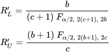
- where F(α/2, n, d) is a quantile from the F distribution with n and d degrees of freedom.
You should use the exact test for analysis; McNemar's test is included for interest only.
If you need the exact confidence interval for the difference between a pair of proportions then please see paired proportions.
DATA INPUT:
Observed frequencies should be entered as a paired fourfold table:
|
|
|
Control/reference category: |
|
|
|
|
outcome present |
outcome absent |
|
Case/index category: |
outcome present: |
a |
b |
|
outcome absent: |
c |
d |
|
Example
From Armitage and Berry (1994, p. 127).
The data below represent a comparison of two media for culturing Mycobacterium tuberculosis. Fifty suspect sputum specimens were plated up on both media and the following results were obtained:
|
|
|
Medium B: |
|
|
|
|
Growth |
No Growth |
|
Medium A: |
Growth: |
20 |
12 |
|
|
No Growth: |
2 |
16 |
To analyse these data in StatsDirect you should select the McNemar function from the chi-square section of the analysis menu. Select the default 95% confidence interval. Enter the counts into the table as shown above.
For this example:
Uncorrected Chi² = 7.142857 (1 DF) P = 0.0075
Yates' continuity corrected Chi² = 5.785714 (1 DF) P = 0.0162
After Liddell (1983):
Point estimate of relative risk (R') = 6
Exact 95% confidence interval = 1.335744 to 55.197091
F = 4, two sided P = 0.0129
R' is significantly different from unity
Here we can conclude that the tubercle bacilli in the experiment grew significantly better on medium A than on medium B. With 95% confidence we can state that the chances of a positive culture are between 1.34 and 55.20 times greater on medium A than on medium B.

 R code
This R code reproduces the example above. It needs no packages and was checked with R 4.6.1. Paste it into R, or save it as a script and run it.
# McNemar and exact (Liddell) test for matched pairs: the StatsDirect help example
# (Armitage and Berry 1994, p. 127, fifty sputum specimens cultured on two media) in R
counts <- matrix(c(20, 12, 2, 16), 2, byrow = TRUE,
                 dimnames = list("Medium A" = c("Growth", "No growth"),
                                 "Medium B" = c("Growth", "No growth")))
print(counts)
b <- counts[1, 2]     # discordant pairs: growth on medium A only
cc <- counts[2, 1]    # growth on medium B only (the cell the table above calls c)

# R's standard McNemar test uses only the discordant pairs b and c. Its default,
# correct = TRUE, applies Yates' continuity correction, as the report's second
# chi-square does; correct = FALSE gives the uncorrected chi-square. When b = c, R
# prints 0 for both chi-squares (P = 1).
print(mcnemar.test(counts, correct = FALSE))
print(mcnemar.test(counts))

# Liddell's exact test: under the null hypothesis b is binomial from b + c with
# probability 1/2, so binom.test gives the two sided P and the exact
# (Clopper-Pearson) 95% confidence interval for the proportion b/(b + c)
exact <- binom.test(b, b + cc)
print(exact)

# The figures as the report prints them, to 6 places (P values to 4)
six <- function(x) formatC(x, digits = 6, format = "f", drop0trailing = TRUE)
pv <- function(p) {
  if (p < 0.0001) "P < 0.0001" else
    paste("P =", formatC(p, digits = 4, format = "f", drop0trailing = TRUE))
}
chi <- mcnemar.test(counts, correct = FALSE)
yates <- mcnemar.test(counts)
cat("Uncorrected Chi-square =", six(chi$statistic), "(1 DF)  ", pv(chi$p.value), "\n")
cat("Yates' continuity corrected Chi-square =", six(yates$statistic), "(1 DF)  ",
    pv(yates$p.value), "\n")

# R' = b/c is the proportion b/(b + c) expressed as odds, p/(1 - p), so its exact
# interval is the binomial interval transformed the same way. It equals the
# interval the F quantiles above give when b and c are both positive.
odds <- exact$conf.int / (1 - exact$conf.int)
cat("Point estimate of relative risk (R') =", six(b / cc), "\n")
cat("Exact 95% confidence interval =", six(odds[1]), "to", six(odds[2]), "\n")
lower <- b / ((cc + 1) * qf(0.975, 2 * (cc + 1), 2 * b))
upper <- (b + 1) * qf(0.975, 2 * (b + 1), 2 * cc) / cc
cat("  (from the F quantiles:", six(lower), "to", six(upper), ")\n")

# F = b/(c + 1), with b the larger of the two discordant counts, has 2(c + 1) and 2b
# degrees of freedom; twice its upper tail area is the binomial two sided P above
r <- max(b, cc)
s <- min(b, cc)
fstat <- r / (s + 1)
cat("F =", six(fstat), "\n")
cat("Two sided", pv(min(1, 2 * pf(fstat, 2 * (s + 1), 2 * r, lower.tail = FALSE))),
    "\n")