Univariate Summary
Menu locations:
Analysis_Descriptive_Univariate Summary;
Analysis_Descriptive_Weighted Univariate Summary.
This function provides measures of location and dispersion which describe the data in a worksheet column. You are given the number, arithmetic mean, sum, variance, standard deviation, standard error of the arithmetic mean, coefficient of variance, confidence interval for the arithmetic mean, geometric mean, coefficient of skewness, coefficient of kurtosis, maximum, upper quartile, median, lower quartile, minimum and range for each selected variable. You can also choose to calculate an additional quantile and this is appended to the results listed above. Incalculable results are displayed as missing data using an asterisk (*).
If you select more than one column of data to describe then you are given an option to save the results to worksheet columns. Saved columns of results represent the statistics, mean, median etc., and their rows represent the variables/columns you selected to describe.
Confidence limits (boundaries of the confidence interval) are given for the arithmetic mean. Please see quantile confidence interval for confidence intervals for the median and other measures of location.
Some related topics:
- central tendency
- variance, standard deviation and spread
- skewness
- normal distribution
- quantiles
- quantile confidence intervals
- histogram
Please refer to one of the general textbooks listed in the reference sectionfor discussion of the application and relative merits of individual descriptive statistics.
Definitions
Valid data and missing data
For each worksheet column that you select, the number of valid data are the number of cells that can be interpreted as numbers, the remaining cells that can not be interpreted as numbers are counted as missing (e.g. empty cell, asterisk or text label). The sample size used in the calculations below is the number of valid data.
Sum, mean, variance, standard deviation, standard error and variance coefficient
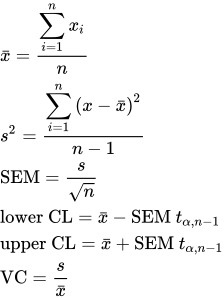
- where Σ is the summation for all observations (xi) in a sample, x bar is the sample (arithmetic) mean, n is the sample size, s² is the sample variance, s is the sample standard deviation, SEM is the standard error of the sample mean, upper and lower CL are the confidence limits of the confidence interval for the mean, tα, n-1 is the (100*a)% two tailed quantile from the Student t distribution with n-1 degrees of freedom, and VC is the variance coefficient.
Skewness and kurtosis
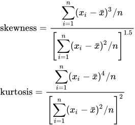
- where Σ is the summation for all observations (xi) in a sample, x bar is the sample mean and n is the sample size. Note that there are other definitions of these coefficients used by some other statistical software. StatsDirect uses the standard definitions for which critical values are published in standard statistical tables (Pearson and Hartley, 1970; Stuart and Ord, 1994).
Geometric mean
The geometric mean is a useful measure of central tendency for samples that are log-normally distributed (i.e. the logarithms of the observations are from an approximately normal distribution). The geometric mean is not calculated for samples that contain values of zero or below.
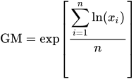
- where Σ is the summation for all observations (xi) in a sample, ln is the natural (base e) logarithm, exp is the exponent (anti-logarithm for base e), GM is the sample geometric mean and n is the sample size.
Weights
If weights are selected then the weights that you supply are first normalised so that they sum to the total number of observations n:
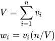
- where vi is a user supplied weight and wi is the normalised weight.
The following formulae replace the mean, variance and moments calculations defined above when weights are used:
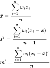
- where mr is the rth moment about the mean; skewness is m3/m21.5 and kurtosis is m4/m22.
Median, quartiles and range
For samples that are not from an approximately normal distribution, for example when data are censored to remove very large and/or very small values, the following nonparametric statistics should be used in place of the arithmetic mean, its variance and the other parametric measures above.
Median (50th centile, quantile 0.5), lower quartile (25th centile, quantile 0.25) and upper quartile (75th centile, quantile 0.75) are defined generally as quantiles:
Two different quantile definitions (Weisberg, 1992; Gleason, 1997; Stuart and Ord, 1994) are used in the summary statistics (see also: quantiles): the first (selected as centile type 2 in the descriptive statistics options) is the conventional quantile that is also used in the quantile confidence interval function and the second (centile type 1, always used for weighted summaries) allows for weights:
Centile type 2:
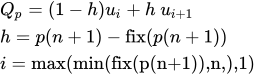
- where p is a proportion, Q is the pth quantile (e.g. median is Q(0.5)), fix is the integer part of a real number, h is the fractional part of order statistic i, u is an observation from a sample after it has been ordered from smallest to largest value and n is the sample size. When i = n the quantile is un (h is then zero, and there is no un+1 to evaluate), so Q(0) = u1 and Q(1) = un.
Centile type 1:
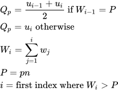
- where p is a proportion, Q is the pth quantile (e.g. median is Q(0.5)), u is an observation from a sample after it has been ordered from smallest to largest value, n is the sample size, w is a weight normalised so that it sums to n and Wi is the sum of the weights of the first i ordered observations. At the two ends, Q(0) is the smallest observation u1 and Q(1) is the largest, un. A single observation is its own median, quartiles and centiles.
Technical validation
The computational methods used in StatsDirect univariate summary statistics, including this function, provide 15 decimal places of precision. This is tested against known standards such as the reference data set used in the example below.
Example
Test workbook (Parametric worksheet: Michelson).
The data are 100 measurements of the speed (millions of meters per second) of light in air recorded by Michelson in 1879 (Dorsey, 1944). The American National Institute of Standards and Technology use these data as part of the Statistical Reference Datasets for testing statistical software (McCullough and Wilson, 1999; http://www.itl.nist.gov/div898/strd/).
Open the test workbook and select the "Michelson" column. Choose Univariate Summary from the Descriptive section of the analysis menu and click on OK when you see a list of descriptive statistics options.
Results from StatsDirect (with decimal places in Analysis_Options set to 12 and centile type 2 selected):
Descriptive statistics
| Variables | Michelson |
| Valid data | 100 |
| Missing data | 0 |
| Sum | 29985.24 |
| Mean | 299.8524 |
| Variance | 0.006242666667 |
| Standard deviation | 0.079010547819 |
| Variance coefficient | 0.000263498134 |
| Standard error of mean | 0.007901054782 |
| Upper 95% CL of mean | 299.868077406834 |
| Lower 95% CL of mean | 299.836722593166 |
| Geometric mean | 299.852389694496 |
| Skewness | -0.018259613963 |
| Kurtosis | 3.263530532311 |
| Maximum | 300.07 |
| Upper quartile | 299.8975 |
| Median | 299.85 |
| Lower quartile | 299.8025 |
| Interquartile range | 0.095 |
| Minimum | 299.62 |
| Range | 0.45 |
| Centile 95 | 299.98 |
| Centile 5 | 299.721 |
Weighted example
Suppose that the five possible responses to a question, 1 to 5, are to be summarised with weights 2, 1, 3, 1 and 1 (an illustration). Enter the values in one column and the weights in another, select Weighted Univariate Summary from the Descriptive section of the Analysis menu, and select the values column and then the weights column. The weights are scaled to sum to the number of values, 5, and n is 5 in the formulae above, so this is not the same as the unweighted summary of eight responses of which two are 1, one is 2 and so on.
| Variables | Value (weight: Frequency) |
| Valid data | 5 |
| Missing data | 0 |
| Sum of weights | 8 |
| Mean | 2.75 |
| Variance | 2.109375 |
| Standard deviation | 1.452369 |
| Variance coefficient | 0.528134 |
| Standard error of mean | 0.649519 |
| Upper 95% CL of mean | 4.553354 |
| Lower 95% CL of mean | 0.946646 |
| Geometric mean | 2.394297 |
| Skewness | 0.1283 |
| Kurtosis | 2.069959 |
| Maximum | 5 |
| Upper quartile | 3.5 |
| Median | 3 |
| Lower quartile | 1.5 |
| Interquartile range | 2 |
| Minimum | 1 |
| Range | 4 |
| Centile 95 | 5 |
| Centile 5 | 1 |

 R code
This R code reproduces the two examples above. It needs no packages and was checked with R 4.6.1. Paste it into R, or save it as a script and run it.
# Univariate summary: the StatsDirect help example (Michelson's 100 measurements
# of the speed of light in air, millions of metres per second) in R
speed <- c(299.85, 299.74, 299.90, 300.07, 299.93, 299.85, 299.95, 299.98, 299.98,
           299.88, 300.00, 299.98, 299.93, 299.65, 299.76, 299.81, 300.00, 300.00,
           299.96, 299.96, 299.96, 299.94, 299.96, 299.94, 299.88, 299.80, 299.85,
           299.88, 299.90, 299.84, 299.83, 299.79, 299.81, 299.88, 299.88, 299.83,
           299.80, 299.79, 299.76, 299.80, 299.88, 299.88, 299.88, 299.86, 299.72,
           299.72, 299.62, 299.86, 299.97, 299.95, 299.88, 299.91, 299.85, 299.87,
           299.84, 299.84, 299.85, 299.84, 299.84, 299.84, 299.89, 299.81, 299.81,
           299.82, 299.80, 299.77, 299.76, 299.74, 299.75, 299.76, 299.91, 299.92,
           299.89, 299.86, 299.88, 299.72, 299.84, 299.85, 299.85, 299.78, 299.89,
           299.84, 299.78, 299.81, 299.76, 299.81, 299.79, 299.81, 299.82, 299.85,
           299.87, 299.87, 299.81, 299.74, 299.81, 299.94, 299.95, 299.80, 299.81,
           299.87)
n <- length(speed)

# R's standard summary, then each statistic of the report, printed to 12 places
# as the example shows them (decimal places set to 12 in Analysis_Options)
print(summary(speed))
twelve <- function(x) {
  formatC(round(x, 12), digits = 12, format = "f", drop0trailing = TRUE)
}
cat("Valid data", n, "  Missing data", sum(is.na(speed)), "\n")
cat("Sum", twelve(sum(speed)), "\n")
cat("Mean", twelve(mean(speed)), "\n")
cat("Variance", twelve(var(speed)), "\n")
cat("Standard deviation", twelve(sd(speed)), "\n")
cat("Variance coefficient", twelve(sd(speed) / mean(speed)), "\n")
se <- sd(speed) / sqrt(n)
cat("Standard error of mean", twelve(se), "\n")
cat("Upper 95% CL of mean", twelve(mean(speed) + qt(0.975, n - 1) * se), "\n")
cat("Lower 95% CL of mean", twelve(mean(speed) - qt(0.975, n - 1) * se), "\n")
cat("Geometric mean", twelve(exp(mean(log(speed)))), "\n")

# Skewness and kurtosis are sqrt(b1) and b2, from the moments about the mean
# with n as the divisor, as in the normality tests
m <- function(k) mean((speed - mean(speed))^k)
cat("Skewness", twelve(m(3) / m(2)^1.5), "\n")
cat("Kurtosis", twelve(m(4) / m(2)^2), "\n")

# Centile type 2 interpolates between the ordered values at p(n + 1): type 6 in
# R, whose default, type 7, interpolates at 1 + p(n - 1) instead
q <- quantile(speed, c(0.05, 0.25, 0.5, 0.75, 0.95), type = 6)
cat("Maximum", max(speed), "\n")
cat("Upper quartile", twelve(q[4]), "\n")
cat("Median", twelve(q[3]), "\n")
cat("Lower quartile", twelve(q[2]), "\n")
cat("Interquartile range", twelve(q[4] - q[2]), "\n")
cat("Minimum", min(speed), "\n")
cat("Range", twelve(max(speed) - min(speed)), "\n")
cat("Centile 95", twelve(q[5]), "\n")
cat("Centile 5", twelve(q[1]), "\n")

# Weighted univariate summary: five values with weights, as a second example.
# StatsDirect first scales the weights to sum to the number of values n, then
# uses n - 1 for the variance and n for the moments and the standard error, so a
# weighted summary is not the summary of the values repeated by their weights.
value <- 1:5
weight <- c(2, 1, 3, 1, 1)
n <- length(value)
w <- weight * n / sum(weight)
m <- weighted.mean(value, w)
v <- sum(w * (value - m)^2) / (n - 1)
six <- function(x) formatC(round(x, 6), digits = 6, format = "f", drop0trailing = TRUE)
cat("Valid data", n, "  Sum of weights", sum(weight), "\n")
cat("Mean", six(m), "  Variance", six(v), "  Standard deviation", six(sqrt(v)), "\n")
cat("Variance coefficient", six(sqrt(v) / m), "  Standard error of mean",
    six(sqrt(v / n)), "\n")
cat("Upper 95% CL of mean", six(m + qt(0.975, n - 1) * sqrt(v / n)),
    "  Lower 95% CL of mean", six(m - qt(0.975, n - 1) * sqrt(v / n)), "\n")
cat("Geometric mean", six(exp(sum(w * log(value)) / n)), "\n")
mom <- function(k) sum(w * (value - m)^k) / n
cat("Skewness", six(mom(3) / mom(2)^1.5), "  Kurtosis", six(mom(4) / mom(2)^2), "\n")

# Centile type 1 with weights: the ordered value at which the cumulative scaled
# weight first exceeds pn, or the average of it and the value before when the
# cumulative weight reaches pn exactly
centile <- function(p) {
  cum <- cumsum(w)
  i <- which(cum > p * n)[1]
  if (i > 1 && isTRUE(all.equal(cum[i - 1], p * n))) (value[i - 1] + value[i]) / 2
  else value[i]
}
cat("Upper quartile", centile(0.75), "  Median", centile(0.5), "  Lower quartile",
    centile(0.25), "  Centile 95", centile(0.95), "  Centile 5", centile(0.05), "\n")