One Way Analysis of Variance
Menu location: Analysis_Analysis of Variance_One Way.
This function compares the sample means for k groups. There is an overall test for k means, multiple comparison methods for pairs of means and tests for the equality of the variances of the groups.
Consider four groups of data that represent one experiment performed on four occasions with ten different subjects each time. You could explore the consistency of the experimental conditions or the inherent error of the experiment by using one way analysis of variance (ANOVA), however, agreement analysis might be more appropriate. One way ANOVA is more appropriate for finding statistical evidence of inconsistency or difference across the means of the four groups.
One way ANOVA assumes that each group comes from an approximately normal distribution and that the variability within the groups is roughly constant. The factors are arranged so that experiments are columns and subjects are rows, this is how you must enter your data in the StatsDirect workbook. The overall F test is fairly robust to small deviations from these assumptions but you could use the Kruskal-Wallis test as an alternative to one way ANOVA if there was any doubt.
Numerically, one way ANOVA is a generalisation of the two sample t test. The F statistic compares the variability between the groups to the variability within the groups:
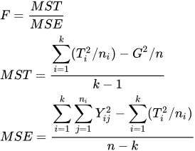
- where F is the variance ratio for the overall test, MST is the mean square due to treatments/groups (between groups), MSE is the mean square due to error (within groups, residual mean square), Yij is an observation, Ti is a group total, G is the grand total of all observations, ni is the number in group i and n is the total number of observations.
Assumptions:
- random samples
- normally distributed observations in each population
- equal variance of observations in each population
- the homogeneity of variance option (marked as "Equality of variance (Levene, Bartlett) and Welch's F" in the ANOVA results window) can be used to test the variance assumption. The Shapiro-Wilk test can be used to look for evidence of non-normality. The most commonly unacceptable deviation from the assumptions is inequality of variance when the groups are of unequal sizes.
A significant overall test indicates a difference between the population means for the groups as a whole; you may then go on to make multiple comparisons between the groups but this "dredging" should be avoided if possible.
If the subjects in this example had been grouped into blocks (for example by litter) before being allocated at random to the treatments, a two way randomized block design ANOVA would have been used.
Example
From Armitage and Berry (1994, p. 214).
Test workbook (ANOVA worksheet: Expt 1, Expt 2, Expt 3, Expt 4).
The following data represent the numbers of worms isolated from the GI tracts of four groups of rats in a trial of carbon tetrachloride as an anthelminthic. These four groups were the control (untreated) groups.
| Expt 1 | Expt 2 | Expt 3 | Expt 4 |
| 279 | 378 | 172 | 381 |
| 338 | 275 | 335 | 346 |
| 334 | 412 | 335 | 340 |
| 198 | 265 | 282 | 471 |
| 303 | 286 | 250 | 318 |
To analyse these data in StatsDirect you must first prepare them in four workbook columns appropriately labelled. Alternatively, open the test workbook using the file open function of the file menu. Then select One Way from the Analysis of Variance section of the analysis menu. Select the columns marked "Expt 1", "Expt 2","Expt 3" and "Expt 4" in one action when prompted for data.
For this example:
One way analysis of variance
Variables: Expt 1, Expt 2, Expt 3, Expt 4
| Source of Variation | Sum Squares | DF | Mean Square |
| Between Groups | 27234.2 | 3 | 9078.066667 |
| Within Groups | 63953.6 | 16 | 3997.1 |
| Corrected Total | 91187.8 | 19 |
F (variance ratio) = 2.271163 P = 0.1195
The null hypothesis that there is no difference in mean worm counts across the four groups is held. If we had rejected this null hypothesis then we would have had to take a close look at the experimental conditions to make sure that all control groups were exposed to the same conditions.
Technical validation
The American National Institute of Standards and Technology provide Statistical Reference Datasets for testing statistical software (McCullough and Wilson, 1999; http://www.itl.nist.gov/div898/strd/). The results below for the SiRstv data set are given to 12 decimal places. The sums of squares and mean squares agree with the certified values exactly; the F ratio, certified as 1.18046237440255, agrees to 11 decimal places, the twelfth being beyond the precision of double precision arithmetic for these data (their deviations from the mean have only four significant figures).
One way analysis of variance
Variables: Instrument 1, Instrument 2, Instrument 3, Instrument 4, Instrument 5
| Source of Variation | Sum Squares | DF | Mean Square |
| Between Groups | 0.0511462616 | 4 | 0.0127865654 |
| Within Groups | 0.21663656 | 20 | 0.010831828 |
| Corrected Total | 0.2677828216 | 24 |
F (variance ratio) = 1.180462374402 P = 0.3494

 R code
This R code reproduces the example and the technical validation above. It needs no packages and was checked with R 4.6.1. Paste it into R, or save it as a script and run it.
# One way analysis of variance: the StatsDirect help example (Armitage and Berry
# 1994, worms recovered from four groups of rats) in R
expt1 <- c(279, 338, 334, 198, 303)
expt2 <- c(378, 275, 412, 265, 286)
expt3 <- c(172, 335, 335, 282, 250)
expt4 <- c(381, 346, 340, 471, 318)
worms <- c(expt1, expt2, expt3, expt4)
group <- factor(rep(c("Expt 1", "Expt 2", "Expt 3", "Expt 4"), each = 5))

# R's standard analysis gives the same table: its "group" line is Between
# Groups and its "Residuals" line is Within Groups
fit <- aov(worms ~ group)
print(summary(fit))

# The report's lines to 6 places
a <- anova(fit)
six <- function(x) {
  formatC(x, digits = 6, format = "f", drop0trailing = TRUE)
}
pv <- function(p) {
  if (p < 0.0001) "P < 0.0001" else
    paste("P =", formatC(p, digits = 4, format = "f", drop0trailing = TRUE))
}
cat("Between Groups", six(a$"Sum Sq"[1]), a$Df[1], six(a$"Mean Sq"[1]), "\n")
cat("Within Groups", six(a$"Sum Sq"[2]), a$Df[2], six(a$"Mean Sq"[2]), "\n")
cat("Corrected Total", six(sum(a$"Sum Sq")), sum(a$Df), "\n")
cat("F (variance ratio) =", six(a$"F value"[1]), " ", pv(a$"Pr(>F)"[1]), "\n")

# The technical validation example: the NIST SiRstv data (five instruments), to
# 12 places as the help shows them. The twelfth decimal place of F is at the
# limit of double precision for these data, as the topic notes.
inst <- c(196.3052, 196.1240, 196.1890, 196.2569, 196.3403,
          196.3042, 196.3825, 196.1669, 196.3257, 196.0422,
          196.1303, 196.2005, 196.2889, 196.0343, 196.1811,
          196.2795, 196.1748, 196.1494, 196.1485, 195.9885,
          196.2119, 196.1051, 196.1850, 196.0052, 196.2090)
instrument <- factor(rep(1:5, each = 5))
b <- anova(aov(inst ~ instrument))
twelve <- function(x) formatC(x, digits = 12, format = "f", drop0trailing = TRUE)
cat("Between Groups", twelve(b$"Sum Sq"[1]), b$Df[1], twelve(b$"Mean Sq"[1]), "\n")
cat("Within Groups", twelve(b$"Sum Sq"[2]), b$Df[2], twelve(b$"Mean Sq"[2]), "\n")
cat("Corrected Total", twelve(sum(b$"Sum Sq")), sum(b$Df), "\n")
cat("F (variance ratio) =", twelve(b$"F value"[1]), " ", pv(b$"Pr(>F)"[1]), "\n")